简述
边缘指像素值急剧变化的位置。对于识别物体而言,边缘起着非常重要的作用。边缘检测的目的是在不损害图像内容的情况下制作一个线图。其方式依然是以卷积为核心操作。
知识点
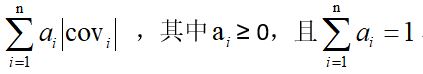
1.有时需要将原图片分别与若干个卷积核进行卷积,这时需要将各个卷积结果进行最终整合,整合的方式主要有以下四种方式
- 取对应位置绝对值的和
- 取对应位置平方和的开方
- 取对应位置绝对值的最大值
- 插值法:
2.因为像素值的范围为0~255,所以图片数组最后的数据类型应该为unit8
Roberts边缘检测
Roberts算子是边缘检测中最简单的算子,利用差分定义生成。
检测流程
1.分别用45°方向差分的卷积算子和135°方向差分的卷积算子对图像进行卷积
2.将上述两个卷积结果进行整合
3.对最后结果进行整理(规范像素值)
说明:
1.scipy库中的convolve2d函数可进行二维数组的卷积,其语法为 scipy.signal.convolve2d(in1, in2, mode='full', boundary='fill', fillvalue=0)
代码示例
import cv2 as cv
import numpy as np
from scipy import signal


# 定义roberts函数
def roberts(I, _boundary='full', _fillvalue=0):
    # 获得原图片的尺寸
    H1, W1 = I.shape[0:2]
    # 定义算子尺寸
    H2, W2 = 2, 2

    # 进行45°方向卷积
    # 定义45°方向卷积核
    R1 = np.array([[1, 0], [0, -1]], np.float32)
    # 锚点位置
    kr1, kc1 = 0, 0
    # 进行卷积
    IconR1 = signal.convolve2d(I, R1, mode='full', boundary=_boundary, fillvalue=_fillvalue)
    # 截取得到same卷积
    IconR1 = IconR1[H2 - kr1 - 1:H1 + H2 - kr1 - 1, W2 - kc1 - 1:W1 + W2 - kc1 - 1]

    # 进行135°方向卷积
    R2 = np.array([[0, 1], [-1, 0]], np.float32)
    kr2, kc2 = 0, 1
    IconR2 = signal.convolve2d(I, R2, mode='full', boundary=_boundary, fillvalue=_fillvalue)
    IconR2 = IconR2[H2 - kr2 - 1:H1 + H2 - kr2 - 1, W2 - kc2 - 1:W1 + W2 - kc2 - 1]

    return (IconR1, IconR2)


if __name__ == "__main__":
    # 读取图片
    image = cv.imread('test2.jpg', flags=0)
    cv.imshow('original_Image', image)

    # 进行roberts边缘检测
    IconR1, IconR2 = roberts(image, 'symm')

    # 取图片数组各值的绝对值
    IconR1 = np.abs(IconR1)
    # RGB图像的深度应为8位
    edge_45 = IconR1.astype(np.uint8)
    cv.namedWindow('edge_45', cv.WINDOW_NORMAL)
    cv.imshow('edge_45', edge_45)

    IconR2 = np.abs(IconR2)
    edge_135 = IconR2.astype(np.uint8)
    cv.namedWindow('edge_135', cv.WINDOW_NORMAL)
    cv.imshow('edge_135', edge_135)

    # 将45°方向卷积结果和135°方向卷积结果平方后求和在开方求得
    edge = np.sqrt(np.power(IconR1, 2.0) + np.power(IconR2, 2.0))
    edge = np.round(edge)
    # 因为是两个图片的‘叠加‘,所以存在大于255的风险,将大于255的像素值都取255
    edge[edge > 255] = 255
    edge = edge.astype(np.uint8)
    cv.namedWindow('edge', cv.WINDOW_NORMAL)
    cv.imshow('edge', edge)

    cv.waitKey()
    cv.destroyAllWindows()


prewitt边缘检测
prewitt算子可以看出是均值平滑算子和Roberts算子卷积后的结果,因此他兼具平滑和检测功能。
检测流程
1.对图像的竖直/水平方向进行平滑
2.对图像的水平/竖直方向进行差分
3.将水平和竖直方向上的差分结果进行整合
4.对最后结果进行整理(规范像素值)
代码示例
import cv2 as cv
import numpy as np
from scipy import signal


def prewitt(I, _boundary='symm'):
    # 先对竖直方向进行平滑
    ones_y = np.array([[1], [1], [1]], np.float32)
    i_conv_pre_x = signal.convolve2d(I, ones_y, mode='same', boundary=_boundary)
    # 再对水平方向进行差分
    diff_x = np.array([[1, 0, -1]], np.float32)
    i_conv_pre_x = signal.convolve2d(i_conv_pre_x, diff_x, mode='same', boundary=_boundary)

    # 对水平方向进行平滑
    ones_x = np.array([[1, 1, 1]], np.float32)
    i_conv_pre_y = signal.convolve2d(I, ones_x, mode='same', boundary=_boundary)
    # 对竖直方向进行差分
    diff_y = np.array([[1], [0], [-1]], np.float32)
    i_conv_pre_y = signal.convolve2d(i_conv_pre_y, diff_y, mode='same', boundary=_boundary)

    return (i_conv_pre_x, i_conv_pre_y)


if __name__ == "__main__":
    # 读取图片,注意,要读入灰度图
    image = cv.imread('test.jpg', flags=0)
    # 显示原图片
    cv.namedWindow('dfs', cv.WINDOW_NORMAL)
    cv.imshow('dfs', image)

    # 调用已写好的函数进行卷积
    i_conv_pre_x, i_conv_pre_y = prewitt(image)

    # 对图像数组的数值取绝对值
    abs_i_conv_pre_x = np.abs(i_conv_pre_x)
    abs_i_conv_pre_y = np.abs(i_conv_pre_y)

    # 重新复制一份结果,后面合成最终结果时会用到
    edge_x = abs_i_conv_pre_x.copy()
    edge_y = abs_i_conv_pre_y.copy()

    # 将超出255的赋值为255
    edge_x[edge_x > 255] = 255
    edge_y[edge_y > 255] = 255

    # 因为色素的数值范围为0~255,所以应该设置为unit8数据类型
    edge_y = edge_y.astype(np.uint8)
    edge_x = edge_x.astype(np.uint8)

    cv.namedWindow('edge_x', cv.WINDOW_NORMAL)
    cv.imshow("edge_x", edge_x)

    cv.namedWindow('edge_y', cv.WINDOW_NORMAL)
    cv.imshow('edge_y', edge_y)

    # 将两个结果合并
    # 有多种合并方法,这里用的时插值法
    edge = abs_i_conv_pre_x * 0.5 + abs_i_conv_pre_y * 0.5
    edge[edge > 255] = 255
    edge = edge.astype(np.uint8)

    cv.namedWindow('edge', cv.WINDOW_NORMAL)
    cv.imshow('edge', edge)
    cv.waitKey()
    cv.destroyAllWindows()


Sobel边缘检测
Sobel算子跟Prewitt算子类似,也自带平滑效果,只不过它的平滑不是非归一均值平滑而是非归一高斯平滑。
检测流程
1.对图像的竖直/水平方向进行平滑
2.对图像的水平/竖直方向进行差分
3.将水平和竖直方向上的差分结果进行整合
4.对最后结果进行整理(规范像素值)
代码示例
import math
import cv2 as cv
import numpy as np
from scipy import signal


# 理论上sobel算法采用高斯平滑的算子,应该比prewitt对“明显”的边缘更加敏感
# 返回n阶非归一化的高斯平滑算子
def pascalSmooth(n):
    # 这里的数组必须为二维,因为后面的convoluted函数要求的输入必须为二维数组
    pascalSmooth = np.zeros([1, n], np.float32)
    for i in range(n):
        # math.factorial(x)函数返回x的阶乘
        pascalSmooth[0][i] = math.factorial(n - 1) / (math.factorial(i) * math.factorial(n - 1 - i))
    return pascalSmooth


# 由高斯平滑算子得到差分算子,并返回差分算子
def pascalDiff(n):
    pascalDiff = np.zeros([1, n], np.float32)
    pascalSmooth_previous = pascalSmooth(n - 1)
    for i in range(n):
        if i == 0:
            pascalDiff[0][i] = pascalSmooth_previous[0][i]
        elif i == n - 1:
            pascalDiff[0][i] = -pascalSmooth_previous[0][i - 1]
        else:
            pascalDiff[0][i] = pascalSmooth_previous[0][i] - pascalSmooth_previous[0][i - 1]
    return pascalDiff


# 得到sobel算子
def getSobelKernel(n):
    pascalSmoothKernel = pascalSmooth(n)
    pascalDiffKernel = pascalDiff(n)
    # np.transpose的功能是将矩阵转置
    sobelKernal_x = signal.convolve2d(pascalSmoothKernel.transpose(), pascalDiffKernel, mode='full')
    sobelKernal_y = signal.convolve2d(pascalSmoothKernel, pascalDiffKernel.transpose(), mode='full')

    return (sobelKernal_x, sobelKernal_y)


# sobel边缘检测核心函数
def sobel(image, n):
    # rows, cols = image.shape
    pascalSmoothKernel = pascalSmooth(n)
    pascalDiffKernel = pascalDiff(n)

    image_sobel_x = signal.convolve2d(image, pascalSmoothKernel.transpose(), mode='same')
    image_sobel_x = signal.convolve2d(image_sobel_x, pascalDiffKernel, mode='same')

    image_sobel_y = signal.convolve2d(image, pascalSmoothKernel, mode='same')
    image_sobel_y = signal.convolve2d(image_sobel_y, pascalDiffKernel.transpose(), mode='same')

    return (image_sobel_x, image_sobel_y)


if __name__ == "__main__":
    image = cv.imread('test4.jpg', flags=0)
    cv.namedWindow('original', cv.WINDOW_NORMAL)
    cv.imshow('original', image)
    # 进行sobel卷积
    sobel_x, sobel_y = sobel(image, 7)
    # 归一化处理
    image_sobel_x = sobel_x / np.max(sobel_x)
    image_sobel_y = sobel_y / np.max(sobel_y)
    image_sobel_x = np.power(image_sobel_x, 1)
    image_sobel_y = np.power(image_sobel_y, 1)
    # 数值化
    image_sobel_x = image_sobel_x * 255
    image_sobel_y = image_sobel_y * 255
    image_sobel_x = image_sobel_x.astype(np.uint8)
    image_sobel_y = image_sobel_y.astype(np.uint8)
    # 显示不同方向的sobel卷积结果
    cv.namedWindow('sobel_x', cv.WINDOW_NORMAL)
    cv.namedWindow('sobel_y', cv.WINDOW_NORMAL)
    cv.imshow('sobel_x', image_sobel_x)
    cv.imshow('sobel_y', image_sobel_y)

    # 对两个方向的处理结果进行整合
    edge = np.sqrt(np.power(sobel_x, 2.0), np.power(sobel_y, 2.0))
    edge = edge / np.max(edge)
    edge *= 255
    edge = edge.astype(np.uint8)
    cv.namedWindow('sobel', cv.WINDOW_NORMAL)
    cv.imshow('sobel', edge)
    cv.waitKey()
    cv.destroyAllWindows()


OpenCV API
函数语法:Sobel( src, ddepth, dx, dy, ksize, scale, borderType )
| 参数 |
解释 |
| src |
输入矩阵 |
| ddepth |
输出矩阵的数据类型 |
| dx |
当dx ≠ 0时,src与差分方向为水平方向上的Sobel核卷积 |
| dy |
当dx = 0,dy ≠ 0时,src与差分方向为垂直方向上的Sobel核卷积 |
| ksize |
Sobel核的尺寸,值为1,3,5,7 |
| Scale(可选) |
比例系数 |
| Delta(可选) |
平移系数 |
| borderType(可选) |
边界扩充类型 |
Canny边缘检测
基于卷积运算的边缘检测算法,如Sobel和Prewitt等有以下两个缺点:
1.没有充分利用边缘的梯度
2.最后输出的边缘二值图只是简单地利用阈值进行处理,容易损失信息。
Canny算法基于这两点做了改进,提出了:
1.基于边缘梯度方向的非极大值抑制
2.双阈值的滞后阈值处理
检测流程
1.高斯平滑去噪
2.计算梯度方向
3.非极大值抑制
4.双阈值的滞后阈值处理
示例代码
import math

import Sobel
import cv2 as cv
import numpy as np


# 非极大值抑制函数,返回“极大值”矩阵
def non_maximum_suppression_default(dx, dy):
    # dx和dy为经过水平差分算子和垂直差分算子卷积后的数值矩阵(sobel或者prewitt)
    edgeMag = np.sqrt(np.power(dx, 2.0), np.power(dy, 2.0))
    rows, cols = edgeMag.shape

    # 梯度矩阵(边缘强度)
    # gradientDirection = np.zeros(edgeMag.shape)
    # 非极大值抑制后的矩阵
    edgeMag_nonMaxSup = np.zeros(edgeMag.shape)

    for r in range(1, rows - 1):
        for c in range(1, cols - 1):
            angle = math.atan2(dy[r][c], dx[r][c]) / math.pi * 180
            # gradientDirection[r][c] = angle
            # 判断差值方向
            # 左右方向
            if (abs(angle) < 22.5 or abs(angle) > 157.5):
                if (edgeMag[r][c] > edgeMag[r][c - 1] and edgeMag[r][c] > edgeMag[r][c + 1]):
                    edgeMag_nonMaxSup[r][c] = edgeMag[r][c]
            # 左上/右下方向
            if (angle >= 22.5 and angle < 67.5 or (-angle > 112.5 and -angle <= 157.5)):
                if (edgeMag[r][c] > edgeMag[r - 1][c - 1] and edgeMag[r][c] > edgeMag[r + 1][c + 1]):
                    edgeMag_nonMaxSup[r][c] = edgeMag[r][c]
            # 上下方向
            if (abs(angle) >= 67.5 and abs(angle) <= 112.5):
                if (edgeMag[r][c] > edgeMag[r - 1][c] and edgeMag[r][c] > edgeMag[r + 1][c]):
                    edgeMag_nonMaxSup[r][c] = edgeMag[r][c]
            # 右上/左下方向
            if ((angle > 112.5 and angle <= 157.5) or (-angle >= 22.5 and -angle < 67.5)):
                if (edgeMag[r][c] > edgeMag[r - 1][c + 1] and edgeMag[r][c] > edgeMag[r + 1][c - 1]):
                    edgeMag_nonMaxSup[r][c] = edgeMag[r][c]

    return edgeMag_nonMaxSup


# 判断一个点的坐标是否在图像内
def checkInRange(r, c, rows, cols):
    if r >= 0 and r < rows and c >= 0 and c < cols:
        return True
    else:
        return False


# 在已有高于阈值点的情况下确定边缘点
def trace(edgeMag_nonMaxSup, edge, lowerThresh, r, c, rows, cols):
    if edge[r][c] == 0:
        # 将符合“边缘”要求的像素值都设置为255
        edge[r][c] = 255
        for i in range(-1, 2):
            for j in range(-1, 2):
                # 大于低阈值便视为边缘
                if checkInRange(r + i, c + j, rows, cols) and edgeMag_nonMaxSup[r + i][c + j] >= lowerThresh:
                    # 这里用递归遍历周围的像素点
                    trace(edgeMag_nonMaxSup, edge, lowerThresh, r + i, c + j, rows, cols)


# 滞后阈值处理
def hyteresisThreshold(edge_nonMaxSup, lowerThresh, upperThresh):
    rows, cols = edge_nonMaxSup.shape
    # 新创建一个用于存储边缘的数组
    edge = np.zeros(edge_nonMaxSup.shape, np.uint8)
    for r in range(1, rows - 1):
        for c in range(1, cols - 1):
            # 如果大于高阈值,就确定与其相连的边缘点
            if edge_nonMaxSup[r][c] >= upperThresh:
                trace(edge_nonMaxSup, edge, lowerThresh, r, c, rows, cols)
            # 如果低于低阈值,就直接舍弃
            if edge_nonMaxSup[r][c] < lowerThresh:
                edge[r][c] = 0
    return edge


if __name__ == "__main__":
    image = cv.imread('test2.jpg', flags=0)
    cv.imshow('original', image)

    image_sobel_x, image_sobel_y = Sobel.sobel(image, 3)
    edge = np.sqrt(np.power(image_sobel_x, 2.0), np.power(image_sobel_y, 2.0))
    edge[edge > 255] = 255
    edge = edge.astype(np.uint8)
    cv.namedWindow('sobel', cv.WINDOW_NORMAL)
    cv.imshow('sobel', edge)

    # 抑制非极大值
    edgeMag_nonMaxSup = non_maximum_suppression_default(image_sobel_x, image_sobel_y)

    edgeMag_nonMaxSup[edgeMag_nonMaxSup > 255] = 255
    edgeMag_nonMaxSup = edgeMag_nonMaxSup.astype(np.uint8)
    cv.namedWindow('edgeMag_nonMaxSup', cv.WINDOW_NORMAL)
    cv.imshow('edgeMag_nonMaxSup', edgeMag_nonMaxSup)

    lowerThresh = 40
    upperThresh = 150
    edge = hyteresisThreshold(edgeMag_nonMaxSup, lowerThresh, upperThresh)
    cv.namedWindow('canny', cv.WINDOW_NORMAL)
    cv.imshow('canny', edge)

    cv.waitKey()
    cv.destroyAllWindows()


OpenCV API
函数语法:Canny(image, edges, threshold1, threshole2, apertureSize, L2gradient )
| 参数 |
解释 |
| image |
输入图像 |
| threshold1 |
低阈值 |
| threshold2 |
高阈值 |
| Edges(可选) |
输出边缘强度图像 |
| apertureSize(可选) |
Sobel核的窗口大小,默认3×3 |
| L2gradient(可选) |
计算总的边缘强度时使用的方式,值为true时代表使用的是平方和开方的方式,值为false代表使用的是绝对值和的方式。 |
Laplacian边缘检测
import cv2 as cv
import numpy as np
from scipy import signal


# 核心步骤,拉普拉斯卷积核与图像矩阵进行卷积
def laplacian(image, _boundary='full', _fillvalue=0):
    laplacianKernel = np.array([[0, -1, 0], [-1, 4, -1], [0, -1, 0]], np.float32)
    i_conv_lap = signal.convolve2d(image, laplacianKernel, mode='same', boundary=_boundary, fillvalue=_fillvalue)

    return i_conv_lap


if __name__ == "__main__":
    image = cv.imread('test5.jpg', flags=0)
    cv.imshow('original', image)
    image = np.array(image)
    # 对图像进行高斯平滑
    image = cv.GaussianBlur(image, (3, 3), 0)
    # 调用拉普拉斯核卷积函数
    threshEdge = laplacian(image, 'symm')

    # 进行阈值处理
    threshEdge[threshEdge > 0] = 255
    threshEdge[threshEdge < 0] = 0
    threshEdge = threshEdge.astype(np.uint8)
    cv.imshow('threshEdge', threshEdge)

    cv.waitKey()
    cv.destroyAllWindows()

OpenCV API
函数语法:placian(src, dst, ddepth, ksize, scale, delta, borderType )
| 参数 |
解释 |
| src |
输入矩阵 |
| dst |
输出矩阵 |
| ddepth |
输出矩阵的数据类型(位深) |
| Ksize(可选) |
Laplacian核的类型 |
| Scale(可选) |
比例系数 |
| delta(可选) |
平移系数 |
| borderType(可选) |
边界扩充类型 |