一、简介
这一节将学习如何定义能够接受多个输入的Keras架构,包括数字,分类和图像数据。 然后,我们将在此混合数据上训练单个端到端网络。
二、从视觉和文本特征估算房价
论文地址:House price estimation from visual and textual features
数据集下载:Dataset
大多数现有的自动房价估算系统仅依赖于一些文本数据,例如其邻近区域和房间数量。最终价格由访问房屋并在视觉上评估房屋的人员估算。在此论文中,他们建议从房屋照片中提取视觉特征,并将它们与房屋的文本信息相结合。这些组合特征被馈送到完全连接的多层神经网络(NN),该网络将房价估算为单一输出。为了训练和评估网络,收集了第一个房屋数据集,它结合了图像和文本属性。该数据集由来自美国加利福尼亚州的535个样本房组成。实验表明,与仅文本特征相比,添加视觉特征使R值增加了3倍,并将均方误差(MSE)降低了一个数量级。此外,在对仅有文本功能的房屋数据集进行培训时,提出的NN仍然优于现有的模型公布结果。这篇论文就是将图像特征和文本特征组合起来,作为网络的输入以提高预测的准确度。
文中采用的方法如图所示:
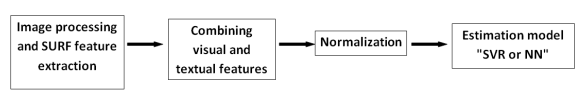
提取图像的SURF特征,将文本特征与之混合,经过归一化处理,最终通过SVR或者NN模型进行预测。
文中的提到的两种模型好坏的评估:
1、均方差损失
均方误差是衡量估计相对于实际数据的接近程度的度量。它测量估计值相对于实际值的误差偏差的平方的平均值。公式如下:

均方差越小,代表模型的可靠度越高。
2、确定系数
确定系数是预测模型相对于实际模型的接近程度的度量。公式如下:
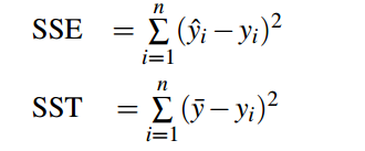
SSE是误差平方和,SST是平方和的总和。确定系数的计算如下:
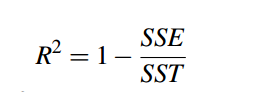
确定系数值越大,表示模型预测的准确性越高。
三、基于CNN与MLP实现数据的混合与多输入
数据准备:
# import the necessary packages
from sklearn.preprocessing import LabelBinarizer
from sklearn.preprocessing import MinMaxScaler
import pandas as pd
import numpy as np
import glob
import cv2
import os

def load_house_attributes(inputPath):
	# initialize the list of column names in the CSV file and then
	# load it using Pandas
	cols = ["bedrooms", "bathrooms", "area", "zipcode", "price"]
	df = pd.read_csv(inputPath, sep=" ", header=None, names=cols)

	# determine (1) the unique zip codes and (2) the number of data
	# points with each zip code
	zipcodes = df["zipcode"].value_counts().keys().tolist()
	counts = df["zipcode"].value_counts().tolist()

	# loop over each of the unique zip codes and their corresponding
	# count
	for (zipcode, count) in zip(zipcodes, counts):
		# the zip code counts for our housing dataset is *extremely*
		# unbalanced (some only having 1 or 2 houses per zip code)
		# so let's sanitize our data by removing any houses with less
		# than 25 houses per zip code
		if count < 25:
			idxs = df[df["zipcode"] == zipcode].index
			df.drop(idxs, inplace=True)

	# return the data frame
	return df

def process_house_attributes(df, train, test):
	# initialize the column names of the continuous data
	continuous = ["bedrooms", "bathrooms", "area"]

	# performin min-max scaling each continuous feature column to
	# the range [0, 1]
	cs = MinMaxScaler()
	trainContinuous = cs.fit_transform(train[continuous])
	testContinuous = cs.transform(test[continuous])

	# one-hot encode the zip code categorical data (by definition of
	# one-hot encoing, all output features are now in the range [0, 1])
	zipBinarizer = LabelBinarizer().fit(df["zipcode"])
	trainCategorical = zipBinarizer.transform(train["zipcode"])
	testCategorical = zipBinarizer.transform(test["zipcode"])

	# construct our training and testing data points by concatenating
	# the categorical features with the continuous features
	trainX = np.hstack([trainCategorical, trainContinuous])
	testX = np.hstack([testCategorical, testContinuous])

	# return the concatenated training and testing data
	return (trainX, testX)

def load_house_images(df, inputPath):
	# initialize our images array (i.e., the house images themselves)
	images = []

	# loop over the indexes of the houses
	for i in df.index.values:
		# find the four images for the house and sort the file paths,
		# ensuring the four are always in the *same order*
		basePath = os.path.sep.join([inputPath, "{}_*".format(i + 1)])
		housePaths = sorted(list(glob.glob(basePath)))

		# initialize our list of input images along with the output image
		# after *combining* the four input images
		inputImages = []
		outputImage = np.zeros((64, 64, 3), dtype="uint8")

		# loop over the input house paths
		for housePath in housePaths:
			# load the input image, resize it to be 32 32, and then
			# update the list of input images
			image = cv2.imread(housePath)
			image = cv2.resize(image, (32, 32))
			inputImages.append(image)

		# tile the four input images in the output image such the first
		# image goes in the top-right corner, the second image in the
		# top-left corner, the third image in the bottom-right corner,
		# and the final image in the bottom-left corner
		outputImage[0:32, 0:32] = inputImages[0]
		outputImage[0:32, 32:64] = inputImages[1]
		outputImage[32:64, 32:64] = inputImages[2]
		outputImage[32:64, 0:32] = inputImages[3]

		# add the tiled image to our set of images the network will be
		# trained on
		images.append(outputImage)

	# return our set of images
	return np.array(images)
模型建立:
# import the necessary packages
from keras.models import Sequential
from keras.layers.normalization import BatchNormalization
from keras.layers.convolutional import Conv2D
from keras.layers.convolutional import MaxPooling2D
from keras.layers.core import Activation
from keras.layers.core import Dropout
from keras.layers.core import Dense
from keras.layers import Flatten
from keras.layers import Input
from keras.models import Model

def create_mlp(dim, regress=False):
	# define our MLP network
	model = Sequential()
	model.add(Dense(8, input_dim=dim, activation="relu"))
	model.add(Dense(4, activation="relu"))

	# check to see if the regression node should be added
	if regress:
		model.add(Dense(1, activation="linear"))

	# return our model
	return model

def create_cnn(width, height, depth, filters=(16, 32, 64), regress=False):
	# initialize the input shape and channel dimension, assuming
	# TensorFlow/channels-last ordering
	inputShape = (height, width, depth)
	chanDim = -1

	# define the model input
	inputs = Input(shape=inputShape)

	# loop over the number of filters
	for (i, f) in enumerate(filters):
		# if this is the first CONV layer then set the input
		# appropriately
		if i == 0:
			x = inputs

		# CONV => RELU => BN => POOL
		x = Conv2D(f, (3, 3), padding="same")(x)
		x = Activation("relu")(x)
		x = BatchNormalization(axis=chanDim)(x)
		x = MaxPooling2D(pool_size=(2, 2))(x)

	# flatten the volume, then FC => RELU => BN => DROPOUT
	x = Flatten()(x)
	x = Dense(16)(x)
	x = Activation("relu")(x)
	x = BatchNormalization(axis=chanDim)(x)
	x = Dropout(0.5)(x)

	# apply another FC layer, this one to match the number of nodes
	# coming out of the MLP
	x = Dense(4)(x)
	x = Activation("relu")(x)

	# check to see if the regression node should be added
	if regress:
		x = Dense(1, activation="linear")(x)

	# construct the CNN
	model = Model(inputs, x)

	# return the CNN
	return model
数据混合输入与训练:
# USAGE
# python mixed_training.py --dataset Houses-dataset/Houses\ Dataset/

# import the necessary packages
from pyimagesearch import datasets
from pyimagesearch import models
from sklearn.model_selection import train_test_split
from keras.layers.core import Dense
from keras.models import Model
from keras.optimizers import Adam
from keras.layers import concatenate
import numpy as np
import argparse
import locale
import os

# construct the argument parser and parse the arguments
ap = argparse.ArgumentParser()
ap.add_argument("-d", "--dataset", type=str, default="D:\Python\opencv\multi-input\Houses Dataset",
	help="path to input dataset of house images")
args = vars(ap.parse_args())

# construct the path to the input .txt file that contains information
# on each house in the dataset and then load the dataset
print("[INFO] loading house attributes...")
inputPath = os.path.sep.join([args["dataset"], "HousesInfo.txt"])
df = datasets.load_house_attributes(inputPath)

# load the house images and then scale the pixel intensities to the
# range [0, 1]
print("[INFO] loading house images...")
images = datasets.load_house_images(df, args["dataset"])
images = images / 255.0

# partition the data into training and testing splits using 75% of
# the data for training and the remaining 25% for testing
print("[INFO] processing data...")
split = train_test_split(df, images, test_size=0.25, random_state=42)
(trainAttrX, testAttrX, trainImagesX, testImagesX) = split

# find the largest house price in the training set and use it to
# scale our house prices to the range [0, 1] (will lead to better
# training and convergence)
maxPrice = trainAttrX["price"].max()
trainY = trainAttrX["price"] / maxPrice
testY = testAttrX["price"] / maxPrice

# process the house attributes data by performing min-max scaling
# on continuous features, one-hot encoding on categorical features,
# and then finally concatenating them together
(trainAttrX, testAttrX) = datasets.process_house_attributes(df,
	trainAttrX, testAttrX)

# create the MLP and CNN models
mlp = models.create_mlp(trainAttrX.shape[1], regress=False)
cnn = models.create_cnn(64, 64, 3, regress=False)

# create the input to our final set of layers as the *output* of both
# the MLP and CNN
combinedInput = concatenate([mlp.output, cnn.output])

# our final FC layer head will have two dense layers, the final one
# being our regression head
x = Dense(4, activation="relu")(combinedInput)
x = Dense(1, activation="linear")(x)

# our final model will accept categorical/numerical data on the MLP
# input and images on the CNN input, outputting a single value (the
# predicted price of the house)
model = Model(inputs=[mlp.input, cnn.input], outputs=x)

# compile the model using mean absolute percentage error as our loss,
# implying that we seek to minimize the absolute percentage difference
# between our price *predictions* and the *actual prices*
opt = Adam(lr=1e-3, decay=1e-3 / 200)
model.compile(loss="mean_absolute_percentage_error", optimizer=opt)

# train the model
print("[INFO] training model...")
model.fit(
	[trainAttrX, trainImagesX], trainY,
	validation_data=([testAttrX, testImagesX], testY),
	epochs=200, batch_size=8)

# make predictions on the testing data
print("[INFO] predicting house prices...")
preds = model.predict([testAttrX, testImagesX])

# compute the difference between the *predicted* house prices and the
# *actual* house prices, then compute the percentage difference and
# the absolute percentage difference
diff = preds.flatten() - testY
percentDiff = (diff / testY) * 100
absPercentDiff = np.abs(percentDiff)

# compute the mean and standard deviation of the absolute percentage
# difference
mean = np.mean(absPercentDiff)
std = np.std(absPercentDiff)

# finally, show some statistics on our model
locale.setlocale(locale.LC_ALL, "en_US.UTF-8")
print("[INFO] avg. house price: {}, std house price: {}".format(
	locale.currency(df["price"].mean(), grouping=True),
	locale.currency(df["price"].std(), grouping=True)))
print("[INFO] mean: {:.2f}%, std: {:.2f}%".format(mean, std))
训练结果:

在整个训练过程中LOSS是连续下降最终收敛,此处只贴出最后一个Epoch的结果图。在经过200个Epoch训练后,我们在测试集上获得了22.41%的误差百分比,这意味着平均而言,我们的网络在其房价预测中将降低约22%的误差。总而言之,这个结果比单独的CNN和MLP效果好,这也是一个简单易懂的数据混合输入的例子。以上就是全部内容,希望大家批评指正!