人工智能 实验5.Hopfield神经网络

版权声明：本文为博主原创文章，转载请声明原创网址。 https://blog.csdn.net/lagoon_lala/article/details/89144028

实验五 Hopfield神经网络

Keras中文文档：https://keras.io/zh/models/sequential/

一、实验目的与要求

1）掌握离散型Hopfield神经网络的原理和网络结构。

2）了解Hopfield神经网络的应用和优化方法。

二、实验内容

1）离散Hopfield神经网络的实现，给记忆样本加30%的噪声，再根据hopfield的特性循环n次，实现记忆样本的还原。

记忆样本，4个5x5的矩阵（来源于网络，分别表示字母N，E，R，0）：

sample =  [[1,-1,-1,-1,1,

           1,1,-1,-1,1,

           1,-1,1,-1,1,

           1,-1,-1,1,1,

           1,-1,-1,-1,1],

          [1,1,1,1,1,

           1,-1,-1,-1,-1,

           1,1,1,1,1,

           1,-1,-1,-1,-1,

           1,1,1,1,1],

          [1,1,1,1,-1,

           1,-1,-1,-1,1,

           1,1,1,1,-1,

           1,-1,-1,1,-1,

           1,-1,-1,-1,1],

          [-1,1,1,1,-1,

           1,-1,-1,-1,1,

           1,-1,-1,-1,1,

           1,-1,-1,-1,1,

           -1,1,1,1,-1]]

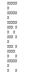
实现的最后结果应该是： 从上到下，第一张为记忆样本、第二张为加噪的记忆样本、第三张为循环n（可设具体数值，比如2000等）次后回忆出的结果。

代码实例：

#1.根据Hebb学习规则计算神经元之间的连接权值 def calcWeight(savedsample):     N = len(savedsample[0])     P = len(savedsample)     mat = [0]*N     returnMat = []     for i in range(N):         m = mat[:]         returnMat.append(m)     for i in range(N):         for j in range(N):             if i==j:                 continue             sum = 0             for u in range(P):                 sum += savedsample[u][i] * savedsample[u][j]             returnMat[i][j] = sum/float(N) return returnMat   #2. 根据神经元的输入计算神经元的输出（静态突触） def calcXi(inMat , weighMat):     returnMat = inMat     choose = []     for i in range(len(inMat)/5):         #随机改变N/5个神经元的值，该参数可调，也可同时改变所有神经元的值         choose.append(random.randint(0,len(inMat)-1))     for i in choose:         sum = 0         for j in range(len(inMat)):             sum += weighMat[i][j] * inMat[j]         if sum>=0:             returnMat[i] = 1         else: returnMat[i] = -1 return returnMat #记忆样本 sample =  [[1,-1,-1,-1,1,            1,1,-1,-1,1,            1,-1,1,-1,1,            1,-1,-1,1,1,            1,-1,-1,-1,1],           [1,1,1,1,1,            1,-1,-1,-1,-1,            1,1,1,1,1,            1,-1,-1,-1,-1,            1,1,1,1,1],           [1,1,1,1,-1,            1,-1,-1,-1,1,            1,1,1,1,-1,            1,-1,-1,1,-1,            1,-1,-1,-1,1],           [-1,1,1,1,-1,            1,-1,-1,-1,1,            1,-1,-1,-1,1,            1,-1,-1,-1,1,            -1,1,1,1,-1]] #加噪函数，在记忆样本的基础上增加30%的噪声 def addnoise(mytest_data,n):     for x in range(n):         for y in range(n):             if random.randint(0, 10) > 7:                 mytest_data[x * n + y] = -mytest_data[x * n + y] return mytest_data #对样本测试，进行记忆样本的迭代和还原： #请输入代码

 

2）（选做题）回忆起原始图片。通过Hopfield神经网络存储一张二值图片，根据某个阈值色度可将每一张图片导出为0-1图片。利用输入的训练图片，获得权重矩阵，或者耦合系数矩阵之后，将该记忆矩阵保存。对图片进行加噪，依然将图片矩阵化，得到二值矩阵。进行迭代，最后，测试图片迭代至稳态或者亚稳态，此时的状态即可认为网络已回忆起原始图片。

图像实例：

 

 

测试图像：

 

代码实现

#导入库，包 import numpy as np import random from PIL import Image import os import re import matplotlib.pyplot as plt from IPython.core.interactiveshell import InteractiveShell InteractiveShell.ast_node_interactivity = "all"   #将jpg格式或者jpeg格式的图片转换为二值矩阵。先生成x这个全零矩阵，从而将imgArray中的色度值分类，获得最终的二值矩阵。 def readImg2array(file,size, threshold= 145):     #file is jpg or jpeg pictures     #size is a 1*2 vector,eg (40,40)     pilIN = Image.open(file).convert(mode="L")     pilIN= pilIN.resize(size)     #pilIN.thumbnail(size,Image.ANTIALIAS)     imgArray = np.asarray(pilIN,dtype=np.uint8)     x = np.zeros(imgArray.shape,dtype=np.float)     x[imgArray > threshold] = 1     x[x==0] = -1     return x   #逆变换 def array2img(data, outFile = None):       #data is 1 or -1 matrix     y = np.zeros(data.shape,dtype=np.uint8)     y[data==1] = 255     y[data==-1] = 0     img = Image.fromarray(y,mode="L")     if outFile is not None:         img.save(outFile)     return img   #利用x.shape得到矩阵x的每一维个数，从而得到m个元素的全零向量。将x按i\j顺序赋值给向量tmp1. 最后得到从矩阵转换的向量。 def mat2vec(x):     #x is a matrix     m = x.shape[0]*x.shape[1]     tmp1 = np.zeros(m)       c = 0     for i in range(x.shape[0]):         for j in range(x.shape[1]):             tmp1[c] = x[i,j]             c +=1 return tmp1   #创建权重矩阵根据权重矩阵的对称特性，可以很好地减少计算量。 #请填写代码   #输入test picture之后对神经元的随机升级。利用异步更新，获取更新后的神经元向量以及系统能量。 #randomly update def update_asynch(weight,vector,theta=0.5,times=100):     energy_ = []     times_ = []     energy_.append(energy(weight,vector))     times_.append(0)     for i in range(times):         length = len(vector)         update_num = random.randint(0,length-1)         next_time_value = np.dot(weight[update_num][:],vector) - theta         if next_time_value>=0:             vector[update_num] = 1         if next_time_value<0:             vector[update_num] = -1         times_.append(i)         energy_.append(energy(weight,vector))         return (vector,times_,energy_) #为了更好地看到迭代对系统的影响，我们按照定义计算每一次迭代后的系统能量，最后画出E的图像，便可验证。   def energy(weight,x,bias=0): #weight: m*m weight matrix #x: 1*m data vector #bias: outer field     energy = -x.dot(weight).dot(x.T)+sum(bias*x)     # E is a scalar     return energy #调用前文定义的函数把主函数表达清楚。可以调整size和threshod获得更好的输入效果为了增加泛化能力，正则化之后打开训练图片，并且通过该程序获取权重矩阵。 #请输入代码 #测试图片 #请输入代码 利用对测试图片的矩阵（神经元状态矩阵）进行更新迭代，直到满足我们定义的迭代次数。最后将迭代末尾的矩阵转换为二值图片输出。 #plt.show()     oshape = matrix_test.shape     aa = update_asynch(weight=w_,vector=vector_test,theta = 0.5 ,times=8000)     vector_test_update = aa[0]     matrix_test_update = vector_test_update.reshape(oshape)     #matrix_test_update.shape     #print(matrix_test_update)     plt.subplot(222)     plt.imshow(array2img(matrix_test_update))     plt.title("recall"+str(num))       #plt.show()     plt.subplot(212)     plt.plot(aa[1],aa[2])     plt.ylabel("energy")     plt.xlabel("update times")         plt.show()

 代码实验1

# -*- coding: utf-8 -*-
import random
#1.根据Hebb学习规则计算神经元之间的连接权值
#Hebb学习规则是一个无监督学习规则，这种学习的结果是使网络能够提取训练集的统计特性，从而把输入信息按照它们的相似性程度划分为若干类。
#即根据事物的统计特征进行分类。Hebb学习规则只根据神经元连接间的激活水平改变权值，因此这种方法又称为相关学习或并联学习。
#Hebb的理论认为在同一时间被激发的神经元间的联系会被强化
def calcWeight(savedsample):
    N = len(savedsample[0])#一个字母的存储长度
    P = len(savedsample)#存储的字母个数
    mat = [0]*N#mat矩阵与一个字母矩阵大小同，全置为0
    returnMat = []#返回矩阵为n*mat
    for i in range(N):
        m = mat[:]
        returnMat.append(m)
    for i in range(N):
        for j in range(N):
            if i==j:
                continue#相同位置为0
            sum = 0
            for u in range(P):#遍历各个矩阵中对应的这两位置
                sum += savedsample[u][i] * savedsample[u][j]
            returnMat[i][j] = sum/float(N)#i->j的权值为各[i]*[j]/N
    return returnMat

#2. 根据神经元的输入计算神经元的输出（静态突触）
def calcXi(inMat , weighMat):
    returnMat = inMat
    choose = []
    #随机回忆N/5个神经元的值，该参数可调，也可同时改变所有神经元的值
    for i in range(int(len(inMat)/5)):
        choose.append(random.randint(0,len(inMat)-1))
    for i in choose:
        sum = 0
        for j in range(len(inMat)):#遍历i到所有输入像素
            sum += weighMat[i][j] * inMat[j]
        if sum>=0:
            returnMat[i] = 1
        else: returnMat[i] = -1
    return returnMat
#加噪函数，在记忆样本的基础上增加30%的噪声
def addnoise(mytest_data,n):
    for x in range(n):#行
        for y in range(n):#列
            if random.randint(0, 10) > 7:#30%
                mytest_data[x * n + y] = -mytest_data[x * n + y]
    return mytest_data

#显示输出
def regularout(data,N):
    for j in range(N):
        ch = ""
        for i in range(N):
            ch += " " if data[j*N+i] == -1 else "X"
        print(ch)

#记忆样本
sample =  [[1,-1,-1,-1,1,
           1,1,-1,-1,1,
           1,-1,1,-1,1,
           1,-1,-1,1,1,
           1,-1,-1,-1,1],
          [1,1,1,1,1,
           1,-1,-1,-1,-1,
           1,1,1,1,1,
           1,-1,-1,-1,-1,
           1,1,1,1,1],
          [1,1,1,1,-1,
           1,-1,-1,-1,1,
           1,1,1,1,-1,
           1,-1,-1,1,-1,
           1,-1,-1,-1,1],
          [-1,1,1,1,-1,
           1,-1,-1,-1,1,
           1,-1,-1,-1,1,
           1,-1,-1,-1,1,
           -1,1,1,1,-1]]
weightMat = calcWeight(sample)
#for i in range(4):
#    regularout(sample[i],5)
regularout(sample[1],5)
test = addnoise(sample[1],5)
regularout(test,5)
for i in range(2000):
    test = calcXi(test,weightMat)
regularout(test,5)

实验二代码

如果报错PIL not named
需要conda install Pillow

# -*- coding: utf-8 -*-
"""
Created on Thu Apr  4 08:28:58 2019

@author: admin
"""

import numpy as np
import random
from PIL import Image
import os
import re
import matplotlib.pyplot as plt
from IPython.core.interactiveshell import InteractiveShell
InteractiveShell.ast_node_interactivity = "all"

#将jpg格式或者jpeg格式的图片转换为二值矩阵。先生成x这个全零矩阵，从而将imgArray中的色度值分类，获得最终的二值矩阵。
def readImg2array(file,size, threshold= 145):
    #file is jpg or jpeg pictures
    #size is a 1*2 vector,eg (40,40)
    pilIN = Image.open(file).convert(mode="L")
    pilIN= pilIN.resize(size)
    #pilIN.thumbnail(size,Image.ANTIALIAS)
    imgArray = np.asarray(pilIN,dtype=np.uint8)
    x = np.zeros(imgArray.shape,dtype=np.float)
    x[imgArray > threshold] = 1
    x[x==0] = -1
    return x

def create_W_single_pattern(x):
    # x is a vector
    if len(x.shape) != 1:
        print ("The input is not vector")
        return
    else:
        w = np.zeros([len(x),len(x)])
        for i in range(len(x)):
            for j in range(i,len(x)):
                if i == j:
                    w[i,j] = 0
                else:
                    w[i,j] = x[i]*x[j]
                    w[j,i] = w[i,j]
    return w
#逆变换
def array2img(data, outFile = None):

    #data is 1 or -1 matrix
    y = np.zeros(data.shape,dtype=np.uint8)
    y[data==1] = 255
    y[data==-1] = 0
    img = Image.fromarray(y,mode="L")
    if outFile is not None:
        img.save(outFile)
    return img

#利用x.shape得到矩阵x的每一维个数，从而得到m个元素的全零向量。将x按i\j顺序赋值给向量tmp1. 最后得到从矩阵转换的向量。
def mat2vec(x):
    #x is a matrix
    m = x.shape[0]*x.shape[1]
    tmp1 = np.zeros(m)

    c = 0
    for i in range(x.shape[0]):
        for j in range(x.shape[1]):
            tmp1[c] = x[i,j]
            c +=1
    return tmp1

#创建权重矩阵根据权重矩阵的对称特性，可以很好地减少计算量。
#请填写代码

#输入test picture之后对神经元的随机升级。利用异步更新，获取更新后的神经元向量以及系统能量。
#randomly update
def update_asynch(weight,vector,theta=0.5,times=100):
    energy_ = []
    times_ = []
    energy_.append(energy(weight,vector))
    times_.append(0)
    for i in range(times):
        length = len(vector)
        update_num = random.randint(0,length-1)
        next_time_value = np.dot(weight[update_num][:],vector) - theta
        if next_time_value>=0:
            vector[update_num] = 1
        if next_time_value<0:
            vector[update_num] = -1
        times_.append(i)
        energy_.append(energy(weight,vector))
    
    return (vector,times_,energy_)
#为了更好地看到迭代对系统的影响，我们按照定义计算每一次迭代后的系统能量，最后画出E的图像，便可验证。

def energy(weight,x,bias=0):
#weight: m*m weight matrix
#x: 1*m data vector
#bias: outer field
    energy = -x.dot(weight).dot(x.T)+sum(bias*x)
    # E is a scalar
    return energy
#调用前文定义的函数把主函数表达清楚。可以调整size和threshod获得更好的输入效果为了增加泛化能力，正则化之后打开训练图片，并且通过该程序获取权重矩阵。
#请输入代码
#测试图片
#请输入代码
#利用对测试图片的矩阵（神经元状态矩阵）进行更新迭代，直到满足我们定义的迭代次数。最后将迭代末尾的矩阵转换为二值图片输出。
#plt.show()
size_global =(80,80)
threshold_global = 60

train_paths = []
#train_path = "/Users/admin/Desktop/train_pics/"
train_path = "train_pics/"
for i in os.listdir(train_path):
    if re.match(r'[0-9 a-z A-Z-_]*.jp[e]*g',i):
        train_paths.append(train_path+i)
flag = 0
for path in train_paths:
    matrix_train = readImg2array(path,size = size_global,threshold=threshold_global)
    vector_train = mat2vec(matrix_train)
    plt.imshow(array2img(matrix_train))
    plt.title("train picture"+str(flag+1))
    plt.show()
    if flag == 0:
        w_ = create_W_single_pattern(vector_train)
        flag = flag +1
    else:
        w_ = w_ +create_W_single_pattern(vector_train)
        flag = flag +1

w_ = w_/flag
print("weight matrix is prepared!!!!!")
test_paths = []
#test_path = "/Users/admin/Desktop/test_pics/"
test_path = "test_pics/"
for i in os.listdir(test_path):
    if re.match(r'[0-9 a-z A-Z-_]*.jp[e]*g',i):
        test_paths.append(test_path+i)
num = 0
for path in test_paths:
    num = num+1
    matrix_test = readImg2array(path,size = size_global,threshold=threshold_global)
    vector_test = mat2vec(matrix_test)
    plt.subplot(221)
    plt.imshow(array2img(matrix_test))
    plt.title("test picture"+str(num))
    oshape = matrix_test.shape
    aa = update_asynch(weight=w_,vector=vector_test,theta = 0.5 ,times=8000)
    vector_test_update = aa[0]
    matrix_test_update = vector_test_update.reshape(oshape)
    #matrix_test_update.shape
    #print(matrix_test_update)
    plt.subplot(222)
    plt.imshow(array2img(matrix_test_update))
    plt.title("recall"+str(num))

    #plt.show()
    plt.subplot(212)
    plt.plot(aa[1],aa[2])
    plt.ylabel("energy")
    plt.xlabel("update times")
    
    plt.show()