1.生成器
1)MRU(SketchyGAN)

计算过程为:
与DCGAN[46]和ResNet生成架构的定性和定量比较可以在5.3节中找到。MRU块有两个输入:输入特征图xi和图像I,输出特征图yi。为了方便起见,我们只讨论输入和输出具有相同空间维数的情况。令[·,·]为串联,Conv(x)为x上的卷积,f(x)为激活函数。我们首先要将输入图像I中的信息合并到输入特征映射xi中。一种幼稚的方法是沿着特征深度维度将它们串联起来并执行卷积:
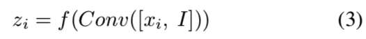
然而,如果块能够在接收到新图像时决定它希望保留多少信息,那就更好了。所以我们采用以下方法:
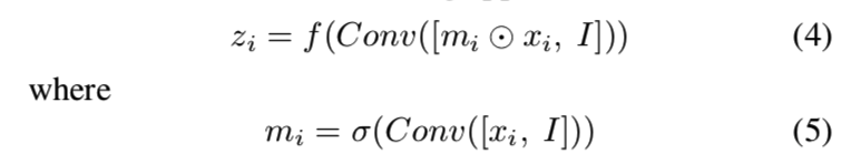
mi是输入特征图上的掩码。可以在这里堆叠多个卷积层以提高性能。然后,我们希望动态地组合来自新卷积的特征图zi和原始输入特征图xi的信息,因此我们使用另一个掩码:

用来将输入特征图和新的特征图连接起来,得到最后的输出:

方程7中的第二项是残差连接。由于有确定信息流的内部掩码,我们称这种结构为掩码残差单元。我们可以将多个这样的单元堆叠起来,重复输入不同的比例的相同的图像,这样网络就可以在其计算路径上动态地从输入图像中检索信息。
2)CSAM(SAGAN)
大多数基于GAN的模型(Radford et al., 2016; Salimans et al., 2016; Karras et al., 2018)使用卷积层构建图像生成。卷积处理一个局部邻域内的信息,因此单独使用卷积层对图像的长期依赖关系建模在计算上是低效的。在本节中,我们采用了(Wang et al., 2018)的非局部模型来介绍GAN框架中的自注意机制,使得生成器和判别器能够有效地对广泛分离的空间区域之间的关系进行建模。因为它的自我注意模块(参见图2),我们将提出的方法称为自注意生成对抗网络(SAGAN)。
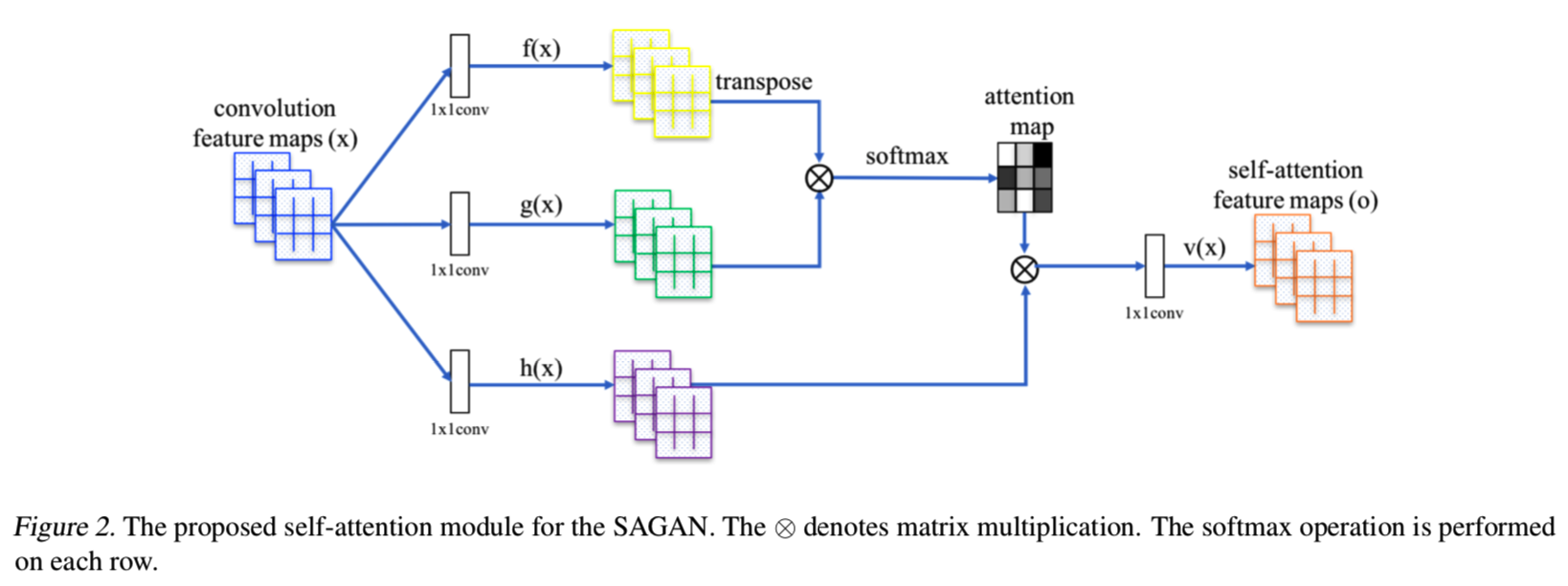
将前一隐含层x∈RC×N的图像特征先变换成两个特征空间f,g来计算注意,其中f (x) = Wfx, g(x) = Wgx:
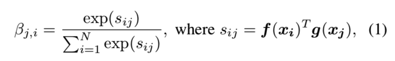
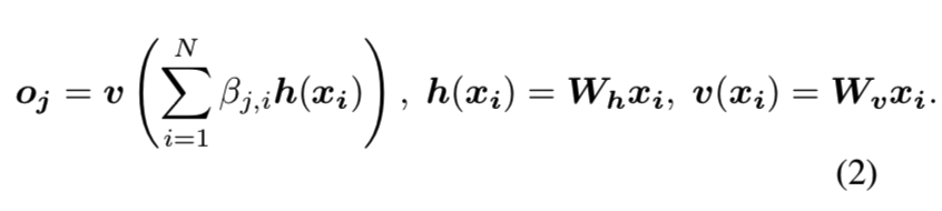
βj,i表示模型在合成第j个区域时对第i个位置的关注程度。其中,C为通道数,N为前一隐含层特征的特征位置数。注意层的输出为o = (o1,o2,…,oj,…,oN)∈RC×N,其中:
在上述公式中,Wg∈RC̄ ×C、Wf∈RC̄ ×C、Wh∈RC̄ ×C和Wv∈RC̄ ×C是可学习的权重矩阵,用来实现1×1的矩阵。在ImageNet的一些迭代后将通道数量从C̄ 减少到C / k, k = 1, 2, 4, 8时,我们没有注意到任何显著的性能下降的。为了提高内存效率,我们选择在我们所有的实验中设置k = 8(即C̄ = C / 8)。
总结一下,CxN = Cx( WxH ),为了进行矩阵相乘所以转换成这个样子,即进行flat操作。通过f(x)、g(x)操作后的输出是[C/8, N],然后对f(x)的结果转置后两者相乘,得到[N, N]大小的s矩阵,表示每个像素点之间的相互关系,可以看成是一个相关性矩阵。h(x)的操作稍微有点不同,输出是[C, N]
然后再使用softmax对s矩阵归一化后得到β矩阵,βj,i表示模型在合成第j像素点时对第i个位置的关注程度,即一个attention map
然后将得到的attention map应用到一个h(x)输出的特征图上,将会对生成的第j个像素造成影响的h(xi)与其对应的影响程度βj,i相乘,然后求和,这就能根据影响程度来生成j像素,将这个结果在进行一层卷积即得到添加上注意的特征图的结果o
此外,我们还将注意力层的输出与比例参数相乘,并将输入的特征图添加回来。因此,最终输出为:
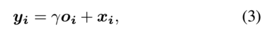
这样得到的结果就是将原来的特征图x加上增加上注意机制的o后的结果
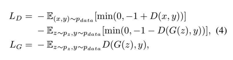
γ是可学习的标量,它初始化为0。首先介绍可学习的γ允许网络依赖在局部领域的线索——因为这更容易,然后逐渐学习分配更多的权重给非局部的证据。我们这样做的直觉很简单:我们想先学习简单的任务,然后逐步增加任务的复杂性。在SAGAN中,提出的注意模块已应用于生成器和判别器,通过最小化铰链式的对抗损失以交替方式进行训练(Lim & Ye, 2017; Tran et al., 2017; Miyato et al., 2018)
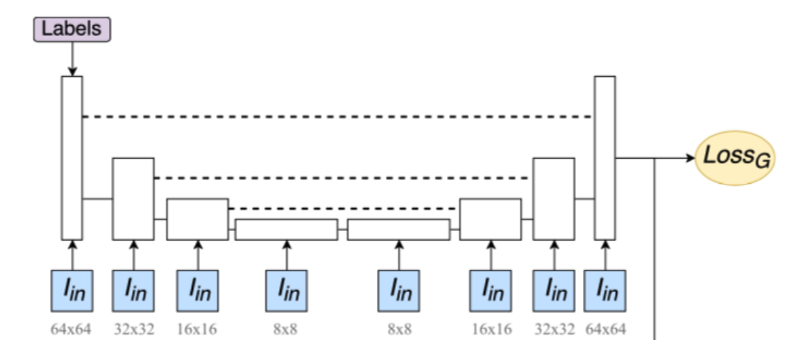
2.多尺度判别器
1)pix2pix
使用的是patch Discriminator
什么是patch Discriminator,比如70*70。之前一直都理解得不对,以为是要将生成的假图像和真图像分成一个个70*70大小的patch输入到判别器中,虽然其实意思就是这个意思,但是实现更加简单。输入还是一整张图片,比如pix2pix中的70*70 patch的判别器的定义为:


import functools
from torch import nn
class NLayerDiscriminator(nn.Module):
    """Defines a PatchGAN discriminator"""

    def __init__(self, input_nc, ndf=64, n_layers=3, norm_layer=nn.BatchNorm2d):
        """Construct a PatchGAN discriminator

        Parameters:
            input_nc (int)  -- the number of channels in input images
            ndf (int)       -- the number of filters in the last conv layer
            n_layers (int)  -- the number of conv layers in the discriminator
            norm_layer      -- normalization layer
        """
        super(NLayerDiscriminator, self).__init__()
        if type(norm_layer) == functools.partial:  # no need to use bias as BatchNorm2d has affine parameters
            use_bias = norm_layer.func == nn.InstanceNorm2d
        else:
            use_bias = norm_layer == nn.InstanceNorm2d

        kw = 4
        padw = 1
        sequence = [nn.Conv2d(input_nc, ndf, kernel_size=kw, stride=2, padding=padw), nn.LeakyReLU(0.2, True)]
        nf_mult = 1
        nf_mult_prev = 1
        for n in range(1, n_layers):  # gradually increase the number of filters
            nf_mult_prev = nf_mult
            nf_mult = min(2 ** n, 8)
            sequence += [
                nn.Conv2d(ndf * nf_mult_prev, ndf * nf_mult, kernel_size=kw, stride=2, padding=padw, bias=use_bias),
                norm_layer(ndf * nf_mult),
                nn.LeakyReLU(0.2, True)
            ]

        nf_mult_prev = nf_mult
        nf_mult = min(2 ** n_layers, 8)
        sequence += [
            nn.Conv2d(ndf * nf_mult_prev, ndf * nf_mult, kernel_size=kw, stride=1, padding=padw, bias=use_bias),
            norm_layer(ndf * nf_mult),
            nn.LeakyReLU(0.2, True)
        ]

        # 最终输出为一个值
        sequence += [nn.Conv2d(ndf * nf_mult, 1, kernel_size=kw, stride=1, padding=padw)]  # output 1 channel prediction map
        self.model = nn.Sequential(*sequence)

    def forward(self, input):
        """Standard forward."""
        return self.model(input)

if __name__ == "__main__":
    d = NLayerDiscriminator(3)
    for module in d.children():
        print(module)
模型为:
Sequential(
  (0): Conv2d(3, 64, kernel_size=(4, 4), stride=(2, 2), padding=(1, 1))
  (1): LeakyReLU(negative_slope=0.2, inplace=True)
  (2): Conv2d(64, 128, kernel_size=(4, 4), stride=(2, 2), padding=(1, 1), bias=False)
  (3): BatchNorm2d(128, eps=1e-05, momentum=0.1, affine=True, track_running_stats=True)
  (4): LeakyReLU(negative_slope=0.2, inplace=True)
  (5): Conv2d(128, 256, kernel_size=(4, 4), stride=(2, 2), padding=(1, 1), bias=False)
  (6): BatchNorm2d(256, eps=1e-05, momentum=0.1, affine=True, track_running_stats=True)
  (7): LeakyReLU(negative_slope=0.2, inplace=True)
  (8): Conv2d(256, 512, kernel_size=(4, 4), stride=(1, 1), padding=(1, 1), bias=False)
  (9): BatchNorm2d(512, eps=1e-05, momentum=0.1, affine=True, track_running_stats=True)
  (10): LeakyReLU(negative_slope=0.2, inplace=True)
  (11): Conv2d(512, 1, kernel_size=(4, 4), stride=(1, 1), padding=(1, 1))
)
可见使用了5层卷积,这五层卷积为:
| layer | kernel size | stride | dilation | padding | input size | output size | receptive field |
| 1 | 4 | 2 | 1 | 1 | 256 | 128 | 70 |
| 2 | 4 | 2 | 1 | 1 | 128 | 64 | 34 |
| 3 | 4 | 2 | 1 | 1 | 64 | 32 | 16 |
| 4 | 4 | 1 | 1 | 1 | 32 | 31 | 7 |
| 5 | 4 | 1 | 1 | 1 | 31 | 30 | 4 |
| output | 30 | 1 |
参考:
https://fomoro.com/research/article/receptive-field-calculator#4,2,1,SAME;4,2,1,SAME;4,2,1,SAME;4,1,1,VALID;4,1,1,VALID
https://github.com/phillipi/pix2pix/blob/master/scripts/receptive_field_sizes.m
https://github.com/junyanz/pytorch-CycleGAN-and-pix2pix/issues/39
感受域的计算为:
def f(output_size, ksize, stride):
    return (output_size - 1) * stride + ksize

if __name__ == "__main__":
    last_layer = f(output_size=1, ksize=4, stride=1)
    # Receptive field: 4
    fourth_layer = f(output_size=last_layer, ksize=4, stride=1)
    # Receptive field: 7
    third_layer = f(output_size=fourth_layer, ksize=4, stride=2)
    # Receptive field: 16
    second_layer = f(output_size=third_layer, ksize=4, stride=2)
    # Receptive field: 34
    first_layer = f(output_size=second_layer, ksize=4, stride=2)
    # Receptive field: 70

    print(first_layer)
意思就是输出中的一个像素一层层往上对应,第五层对应的是4个感受域,第四次对应7个,第三层对应16个,第二层对应34个,第一层对应70个
这样的结构的判别器就是70*70的,该70*70与其输入的图像的大小无关
输出的30*30*1中的每个像素值为其对应的第一层输入的256*256*3中的70*70大小的patch是否为真实图像的判断,因此之后对30*30*1的结果求平均值就能够得到该整体图像是否是真实图像的结果。选择70*70是因为经过实验说明距离超过一个patch直径的像素之间是独立的
因此计算判别器的损失函数为:
class GANLoss(nn.Module):
    """Define different GAN objectives.Gan目标函数

    The GANLoss class abstracts away the need to create the target label tensor
    that has the same size as the input.
    """

    def __init__(self, gan_mode, target_real_label=1.0, target_fake_label=0.0):
        """ Initialize the GANLoss class.

        Parameters:
            gan_mode (str) - - the type of GAN objective. It currently supports vanilla, lsgan, and wgangp.
            target_real_label (bool) - - label for a real image
            target_fake_label (bool) - - label of a fake image

        Note: Do not use sigmoid as the last layer of Discriminator.
        LSGAN needs no sigmoid. vanilla GANs will handle it with BCEWithLogitsLoss.
        """
        super(GANLoss, self).__init__()
        self.register_buffer('real_label', torch.tensor(target_real_label))
        self.register_buffer('fake_label', torch.tensor(target_fake_label))
        self.gan_mode = gan_mode
        if gan_mode == 'lsgan':# 最小二乘法损失
            self.loss = nn.MSELoss()
        elif gan_mode == 'vanilla': # 交叉熵损失
            self.loss = nn.BCEWithLogitsLoss()
        elif gan_mode in ['wgangp']: # 使用梯度惩罚损失,下面的cal_gradient_penalty函数
            self.loss = None
        else:
            raise NotImplementedError('gan mode %s not implemented' % gan_mode)

    def get_target_tensor(self, prediction, target_is_real):
        """Create label tensors with the same size as the input.

        Parameters:
            prediction (tensor) - - tpyically the prediction from a discriminator,用来确定生成的目标值的大小
            target_is_real (bool) - - if the ground truth label is for real images or fake images

        Returns:
            A label tensor filled with ground truth label, and with the size of the input
        """

        if target_is_real: # 如果该预测值prediction对应的应该是个真图,则目标值为true
            target_tensor = self.real_label
        else:# 如果该预测值prediction对应的应该是个假图,则目标值为false
            target_tensor = self.fake_label
        return target_tensor.expand_as(prediction) #这一步最为关键

    def __call__(self, prediction, target_is_real):
        """Calculate loss given Discriminator's output and grount truth labels.

        Parameters:
            prediction (tensor) - - tpyically the prediction output from a discriminator
            target_is_real (bool) - - if the ground truth label is for real images or fake images

        Returns:
            the calculated loss.
        """
        if self.gan_mode in ['lsgan', 'vanilla']:
            target_tensor = self.get_target_tensor(prediction, target_is_real)
            loss = self.loss(prediction, target_tensor) # 计算损失
        elif self.gan_mode == 'wgangp':
            if target_is_real:
                loss = -prediction.mean()
            else:
                loss = prediction.mean()
        return loss
上面标红的那一步就相当于将图的真正标签从1*1*1扩展为判别器的输出结果30*30*1,然后再求损失
2) pix2pixHD
这个则是使用了3个 70*70的patch Discriminator,输入分别为原始图像、下采样一倍的图像和下采样两倍的图像
3) ours
使用了2/3/4个patch Discriminator,不同的patch Discriminator的深度不同,所以感受域也不同,不再是仅使用70*70的情况了,而且深度最大的那个判别器的感受域必须是全局的,用来获得全局信息。而且每个子网在前几层与其他子网共享权重