pytorch学习笔记(一)之线性模型
2020.1.27笔记
- Grad在反向传播过程中是累加的,意味着每一次运行反向传播,梯度都会累加之前的梯度,一般在方向传播之前把梯度清零。
- 不允许张量对张量求导,只允许标量对张量求导,求导结果是和自变量同行的张量。
- 可以用with torch.no_grad()将不想被追踪的操作代码块包裹起来。
- Torch变量带requires_grad的不能进行+=操作。x+=2。
- 批量大小和学习率的值是人为设定的,不是通过模型训练学出的,称之为超参数。
- Python super()函数用于调用父类(超类)的一个方法。
- a.numpy()将a转换成numpy数据类型,torch.from_numpy()将numpy转换为tensor。
- torch.cuda.is_available()判断是否支持gpu,a.cuda()就能够将tensor a放到gpu上面。
- torch.autograd.Variable会被放入计算图中,然后进行前向传播和反向传播,自动求导
包含三个部分data,grad,grad_fn。from torch.autograd import Variable
通过data可以去除variable里面的tensor数值
Grad_fn表示的是得到这个variable的操作
Grad是这个variable反向传播梯度
求导y.backward(),对于标量求导里面的参数可以不写
对于向量求导不能直接写成y.backward()。需要传入参数声明。比如y.backward(torch.FloatTensor([1,1,1])),得到的就是每个分量的梯度。
2020.1.28笔记
- 优化算法:是一种调整模型参数更新的策略
一阶优化算法,使用各个参数的梯度值来更新参数,梯度下降。
二阶优化算法,使用了二阶导数,hessian方法,来最小化或者最大化损失函数。
torch.optim是一个实现各种优化算法的包。在调用时将需要优化的参数传入,这些参数都必须是Variable,然后传入一些基本的设定,比如学习率和动量等。
优化之前,需要先将梯度归0,optimizer.zeros(),然后通过loss.backward()自动求导得到每个参数的梯度,最后只需要optimizer.step()就可以通过梯度做一步参数更新。 - torch.save用于保存模型的结构和参数。保存方式两种:
保存整个模型的结构信息和参数信息,保存的对象是model
保存模型的参数,保存的对象是模型的状态。model.state_dict()。
torch.save(model, ‘./model.pth’)
torch.save(model.state_dict(), ‘./model_state.pth’)
3.加载模型
加载完整的模型结构和参数信息
Load_model = torch.load('model.pth’),网络较大的时候加载时间较长,同时存储空间也比较大。
加载模型参数信息,需要先导入模型的结构,然后
model.load_state_dic(torch.load(‘model_state.pth’))导入。
4.线性回归案例。
给出一系列点,找到拟合的直线。model.eval()将模型变成测试模式,一些层如dropout和batchNormalization在训练和测试的时候是不一样的,因而需要通过这样一个操作来转换这些不一样的层操作。
import torch
from torch import nn,optim
import numpy as np
import matplotlib.pyplot as plt
from torch.autograd import Variable
#线性回归,输入数据(x1,y1),(x2,y2),...,(xn,yn)
x_train = np.array([[3.3],[4.4],[5.5],[6.71],[6.93],[4.168],
                    [9.779],[6.182],[7.59],[2.167],[7.042],
                    [10.791],[5.313],[7.997],[3.1]],dtype=np.float32)
y_train = np.array([[1.7],[2.76],[2.09],[3.19],[1.694],[1.573],
                    [3.366],[2.596],[2.53],[1.221],[2.827],
                    [3.465],[1.65],[2.904],[1.3]],dtype=np.float32)
#转为tensor
x_train = torch.from_numpy(x_train)
y_train = torch.from_numpy(y_train)

#定义线性回归网络结构
class LinearRegression(nn.Module):
    def __init__(self):
        super(LinearRegression, self).__init__()
        self.linear = nn.Linear(1,1)

    def forward(self, x):
        out = self.linear(x)
        return out
#定义在gpu上的LinearRegression成员
if torch.cuda.is_available():
    model = LinearRegression().cuda()
else:
    model = LinearRegression()

#定义损失函数
criterion = nn.MSELoss()
#定义优化函数
optimizer = optim.SGD(model.parameters(), lr=1e-3)
num_epochs = 1000
for epoch in range(num_epochs):
    if torch.cuda.is_available():
        inputs = Variable(x_train).cuda()
        target = Variable(y_train).cuda()
    else:
        inputs = Variable(x_train)
        target = Variable(y_train)
    #forward
    out = model.forward(inputs)
    loss = criterion(out, target)
    #backward
    #梯度清0
    optimizer.zero_grad()
    #反向传播
    loss.backward()
    #参数更新
    optimizer.step()
    if (epoch+1)%40 == 0:
        print('loss:', loss.data)
#将模型转为测试模式
model.eval()
#预测结果
predict = model.forward(Variable(x_train).cuda())
#转成cpu,转为numpy
predict = predict.data.cpu().numpy()
plt.plot(x_train.numpy(), y_train.numpy(), 'ro', label='Original data')
plt.plot(x_train.numpy(), predict, label='Fitting Line')
plt.show()


2020.1.29笔记
多项式回归
- Torch.unsqueeze()对数据维度进行扩充
a.unsqueeze(1)在第二维增加一个维度
torch.squeeze()对数据进行降维,只有维度值为1时才会去掉改维度。 - tensor.size()
import torch
import numpy as np

test = torch.tensor([0,1,2])
print(test.size())
print(test[0], test[1], test[2])

test = torch.tensor([[0,1,2]])
print(test.size())
print(test[0])
print(test[0][0], test[0][1], test[0][2])
运行结果为:
torch.Size([3])
tensor(0) tensor(1) tensor(2)
torch.Size([1, 3])
tensor([0, 1, 2])
tensor(0) tensor(1) tensor(2)
3.torch.mm()为矩阵乘法
x.mm(w_target)
4.
import torch
import numpy as np
from torch import nn, optim
from torch.autograd import Variable
import matplotlib.pyplot as plt
#生成特征点
def make_features(x):
#在第二个维度添加一个维度
#print("before x.size:", x.size())
x = x.unsqueeze(1)
#print("x:", x)
#print("after x.size:", x.size())
return torch.cat([x**i for i in range(1,4)], 1)
w_target = torch.FloatTensor([0.5, 3, 2.4]).unsqueeze(1)
#print('w_target: ', w_target)
b_target = torch.FloatTensor([0.9])
#将每次输入一个x得到一个y的真实函数
def f(x):
return x.mm(w_target) + b_target
#得到batch_size个训练集
def get_batch(batch_size=32):
#生成batch_size个随机数
random = torch.randn(batch_size)
x = make_features(random)
y = f(x)
if torch.cuda.is_available():
return Variable(x).cuda(), Variable(y).cuda()
else:
return Variable(x), Variable(y)
#定义多项式模型
class poly_model(nn.Module):
def __init__(self):
super(poly_model, self).__init__()
#模型输入为3维,输出是1维
self.poly = nn.Linear(3,1)
def forward(self, x):
out = self.poly(x)
return out
def main():
if torch .cuda.is_available():
model = poly_model().cuda()
else:
model = poly_model()
criterion = nn.MSELoss()
#使用随机梯度下降来优化模型
optimizer = optim.SGD(model.parameters(), lr=1e-3)
#开始训练模型
epoch = 0
while True:
# 获取数据集
batch_x, batch_y = get_batch()
#前向传播
output = model.forward(batch_x)
#计算损失
loss = criterion(output, batch_y)
#打印损失值
print_loss = loss.data
#梯度清0
optimizer.zero_grad()
#反向传播
loss.backward()
#更新参数
optimizer.step()
epoch += 1
if print_loss < 1e-3:
break
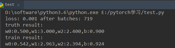
print('loss: %.3f after batches: %d' %(print_loss, epoch))
w_0, w_1, w_2 = model.poly.weight[0]
w_0 = w_0.data.item()
w_1 = w_1.data.item()
w_2 = w_2.data.item()
b_ = model.poly.bias[0].item()
x = np.arange(-1,1,0.1)
w0_truth = w_target[0].item()
w1_truth = w_target[1].item()
w2_truth = w_target[2].item()
b_truth = b_target.item()
y = w0_truth * x + w1_truth * x * x + w2_truth * x * x * x + b_truth
y_ = w_0 * x + w_1 * x * x + w_2 * x * x * x + b_
print('truth result:')
print('w0:%.3f,w1:%.3f,w2:%.3f,b:%.3f' % (w0_truth, w1_truth, w2_truth, b_truth))
print('train result:')
print('w0:%.3f,w1:%.3f,w2:%.3f,b:%.3f' % (w_0, w_1, w_2, b_))
plt.figure()
plt.plot(x, y, 'ro')
plt.plot(x, y_, 'b-')
plt.legend(['actual curve', 'predict curve'])
plt.show()
if __name__ == '__main__':
main()