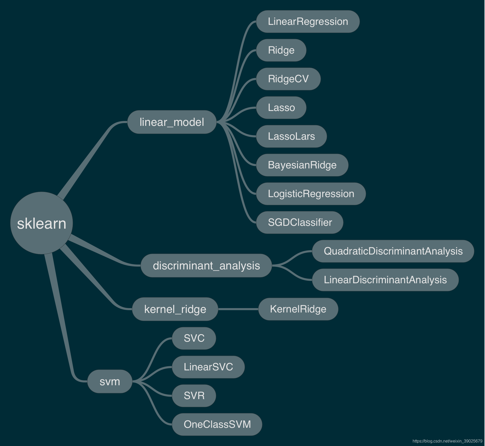
sklearn框架
函数导图
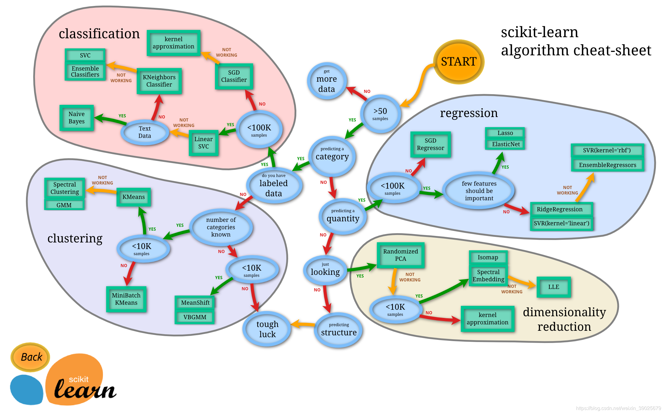
1. Classification
from sklearn import svm
X = [[0, 0], [1, 1]]
y = [0, 1]
clf = svm.SVC()
clf.fit(X, y)
clf.predict([[2., 2.]])
内部参数
# get support vectors
clf.support_vectors_


# get indices of support vectors
clf.support_

# get number of support vectors for each class
clf.n_support_
1.1. Multi-class classification
SVC
X = [[0], [1], [2], [3]]
Y = [0, 1, 2, 3]
clf = svm.SVC(decision_function_shape='ovo')
clf.fit(X, Y)

dec = clf.decision_function([[1]])
dec.shape[1] # 4 classes: 4*3/2 = 6

clf.decision_function_shape = "ovr"
dec = clf.decision_function([[1]])
dec.shape[1] # 4 classes
LinearSVC
lin_clf = svm.LinearSVC()
lin_clf.fit(X, Y)

dec = lin_clf.decision_function([[1]])
dec.shape[1]
1.3. Unbalanced problems
Plot different SVM classifiers in the iris dataset
print(__doc__)

import numpy as np
import matplotlib.pyplot as plt
from sklearn import svm, datasets


def make_meshgrid(x, y, h=.02):
    """Create a mesh of points to plot in

    Parameters
    ----------
    x: data to base x-axis meshgrid on
    y: data to base y-axis meshgrid on
    h: stepsize for meshgrid, optional

    Returns
    -------
    xx, yy : ndarray
    """
    x_min, x_max = x.min() - 1, x.max() + 1
    y_min, y_max = y.min() - 1, y.max() + 1
    xx, yy = np.meshgrid(np.arange(x_min, x_max, h),
                         np.arange(y_min, y_max, h))
    return xx, yy


def plot_contours(ax, clf, xx, yy, **params):
    """Plot the decision boundaries for a classifier.

    Parameters
    ----------
    ax: matplotlib axes object
    clf: a classifier
    xx: meshgrid ndarray
    yy: meshgrid ndarray
    params: dictionary of params to pass to contourf, optional
    """
    Z = clf.predict(np.c_[xx.ravel(), yy.ravel()])
    Z = Z.reshape(xx.shape)
    out = ax.contourf(xx, yy, Z, **params)
    return out


# import some data to play with
iris = datasets.load_iris()
# Take the first two features. We could avoid this by using a two-dim dataset
X = iris.data[:, :2]
y = iris.target

# we create an instance of SVM and fit out data. We do not scale our
# data since we want to plot the support vectors
C = 1.0  # SVM regularization parameter
models = (svm.SVC(kernel='linear', C=C),
          svm.LinearSVC(C=C, max_iter=10000),
          svm.SVC(kernel='rbf', gamma=0.7, C=C),
          svm.SVC(kernel='poly', degree=3, gamma='auto', C=C))
models = (clf.fit(X, y) for clf in models)

# title for the plots
titles = ('SVC with linear kernel',
          'LinearSVC (linear kernel)',
          'SVC with RBF kernel',
          'SVC with polynomial (degree 3) kernel')

# Set-up 2x2 grid for plotting.
fig, sub = plt.subplots(2, 2)
plt.subplots_adjust(wspace=0.4, hspace=0.4)

X0, X1 = X[:, 0], X[:, 1]
xx, yy = make_meshgrid(X0, X1)

for clf, title, ax in zip(models, titles, sub.flatten()):
    plot_contours(ax, clf, xx, yy,
                  cmap=plt.cm.coolwarm, alpha=0.8)
    ax.scatter(X0, X1, c=y, cmap=plt.cm.coolwarm, s=20, edgecolors='k')
    ax.set_xlim(xx.min(), xx.max())
    ax.set_ylim(yy.min(), yy.max())
    ax.set_xlabel('Sepal length')
    ax.set_ylabel('Sepal width')
    ax.set_xticks(())
    ax.set_yticks(())
    ax.set_title(title)

plt.show()
2. Regression
from sklearn import svm
X = [[0, 0], [2, 2]]
y = [0.5, 2.5]
clf = svm.SVR()
clf.fit(X, y)

clf.predict([[1, 1]])
3. Density estimation, novelty detection
The class OneClassSVM implements a One-Class SVM which is used in outlier detection.
from sklearn.svm import OneClassSVM
X = [[0], [0.44], [0.45], [0.46], [1]]
clf = OneClassSVM(gamma='auto').fit(X)
clf.predict(X)

clf.score_samples(X)  # doctest: +ELLIPSIS
6. Kernel functions
6.1. Custom Kernels
6.1.1. Using Python functions as kernels
import numpy as np
from sklearn import svm
def my_kernel(X, Y):
    return np.dot(X, Y.T)

clf = svm.SVC(kernel=my_kernel)
6.1.2. Using the Gram matrix
import numpy as np
from sklearn import svm
X = np.array([[0, 0], [1, 1]])
y = [0, 1]
clf = svm.SVC(kernel='precomputed')
# linear kernel computation
gram = np.dot(X, X.T)
clf.fit(gram, y)

# predict on training examples
clf.predict(gram)
