Binary array conventional beam pattern and its directivity—microphone array series (7)

Read the original text, please move to my knowledge column:
https://www.zhihu.com/column/c_1287066237843951616

The contents of this article are:

Introduction to Binary Array

Example 3.8 Conventional beam pattern of binary array

Example 3.9 Binary array directivity index

Introduction to Binary Array

Figure 1 Binary matrix

Binary array is an array composed of two array elements. Place the first array element at the origin of the coordinates, and the second array element on the $with$ axis. The distance between the two array elements is $d$ . The binary array coordinate system is shown in Figure 1. The position coordinates of the two-element array are:

$\bold p _m=\left[ 0,0,(m-1)d \right]^T,m=1,2$

Due to symmetry, the directivity of the base array has nothing to do with the horizontal azimuth angle, only the pitch angle $\phi$ . Therefore, the array popularity vector of the uniform linear array is:

$\bold p(\phi)=\left[ 1,e^{kdcos\phi} \right]^T$

For this binary matrix, assuming the desired direction is $\ phi_o$ , the weighting vector is:

$\bold w^*\left( \phi_o \right)=\bold p^*\left( \phi_o \right)/2=\left[ 1,e^{-ikdcos\phi_o} \right]^T/2$

Example 3.8 Conventional beam pattern of binary array

This example examines the conventional beam response of a binary array when the distance between the array elements is different.

Assuming that the distance between the array elements is taken from the $d = 0.05 \ lambda, 0.25 \ lambda, 0.5 \ lambda,$ desired beam direction $\ phi_o = 0 ^ \ circ, 60 ^ \ circ, 90 ^ \ circ$ , the calculated conventional beam pattern is shown in the figure $2(a),2(b),2(c)$ . It can be seen from the figure that when the distance between the array elements gradually decreases, the main beam of the binary array becomes wider and the directivity gradually deteriorates. When the distance between the array elements is reduced $d = 0.05 \ lambda$ , the conventional beam pattern of the binary array is close to a circle, that is, it degenerates into a single element without directivity. Observation FIG. 2 (a) found that when $d = 0.25 \ lambda$ , the beam pattern is an inverted "heart-shaped", when the beam weight vector is:

$\bold w^*=\left[ \frac{1}{2}, -\frac{i}{2} \right]^T$

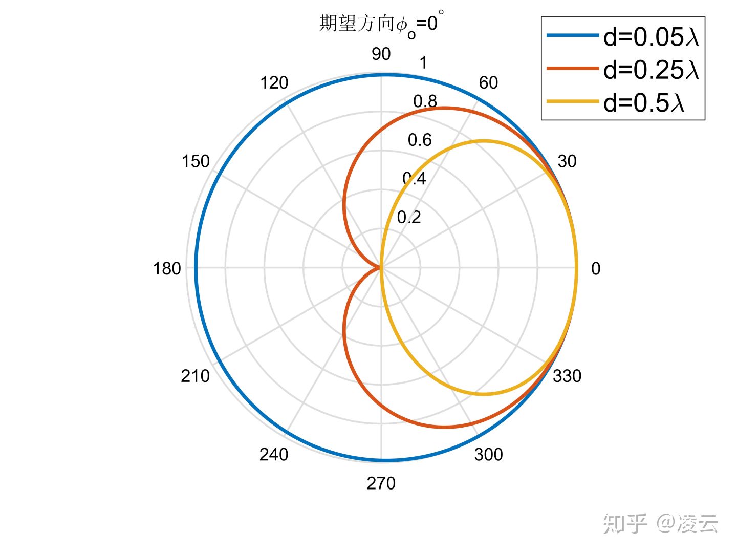
Figure 2(a)

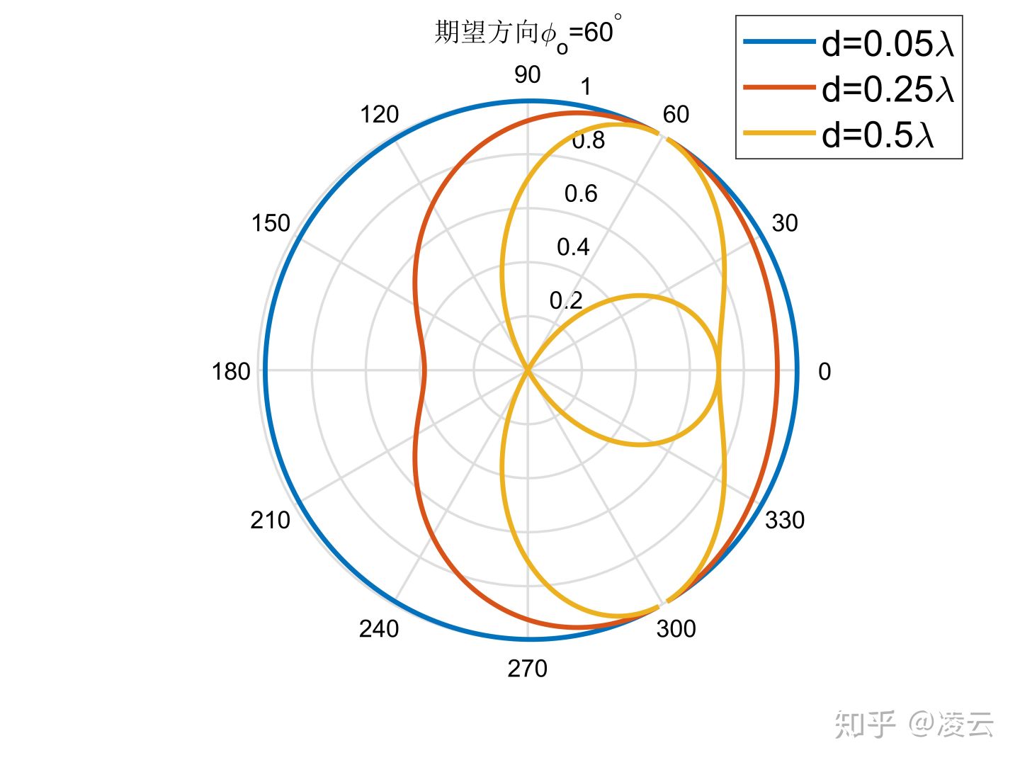
Figure 2(b)

Figure 2(c)

The implementation code is as follows:

f=1000;      %频率
c=340;       %声速
lambda = c/f;
space=0.04;  %麦克风间距
theta_angle=0:1:360;
theta=theta_angle*pi/180;
space_list = [0.05 0.25 0.5]*lambda;  %连续阵间距
M = 2;
figure;
theta_d = 0 *pi/180;
for i = 1:length(space_list)
    space = space_list(i);
    B=sin((M*pi*f*space*(cos(theta)-cos(theta_d)))/c)...
    ./(M*sin((pi*f*space*(cos(theta)-cos(theta_d)))/c));
    B_db=20*log10(B);
    index = B_db < -50;
    B_db(index) = -50;    
    GraphicHandle = polar(theta,B);
    set( GraphicHandle, 'LineWidth', 2);
    hold on;
end
title('期望方向\phi_o=0^\circ');
legend('d=0.05\lambda', 'd=0.25\lambda', 'd=0.5\lambda', 'fontsize', 15);

Example 3.9 Binary array directivity index

The directivity index of the base array The directivity index of the base array is equal to the array gain of the base array in a spatially uniform and isotropic noise field.
Super directivity As the distance between array elements decreases, the directivity of the optimal beam forming of the linear array in the end-fire direction exceeds the number of elements. This status quo is "super directivity" or "super gain".

In this example, consider a binary array. The conventional beamforming method and the optimal beamforming method are used to investigate $\left( d/\lambda \right)$ the directivity index of the basic array under different array element spacing and wavelength ratios and different observation directions.

Suppose the beam direction are observed $\ phi_o = 0 ^ \ circ, 30 ^ \ circ, 60 ^ \ circ, 90 ^ \ circ,$ so that $d / \ lambda$ the $0\sim 0.5$ variation in the range of, respectively, the following equation (3.54) and (3.56)

The gain of the conventional beam formed in the binary array in the spatially uniform and isotropic noise field is:

$Gain_c=\frac{\left| p^Hp \right|^2}{p\rho _{niso}p}=\frac{2}{1+sinc(kd)cos(kdcos\phi)}$

Among them $\ rho_ {nisu}$ is the cross-spectrum matrix of uniform isotropic noise in the binary array space:

$\rho_{niso}=\begin{gathered} \begin{bmatrix} 1 & sinc(kd) \\ sinc(kd) & 1 \end{bmatrix} \quad \end{gathered}$

The optimal beamforming array gain in the binary array in the spatially uniform and isotropic noise field is:

$Gain_{opt}=p^H\rho ^{-1}_{niso}p=\frac{2-2sinc(kd)cos(kdcos\phi)}{1-sinc^2(kd)}$

Calculate the directivity index obtained by the conventional beamforming method and the optimal beamforming method. The directivity calculation results of the two beamforming methods are shown in Figures 3(a) and 3(b), respectively.

Figure 3(a)

As can be seen in FIG. 3 (a), conventional methods for beam forming, as $d / \ lambda = 0.5$ , the directivity $Gain_c=2$ , i.e., the number of array elements. When the beam observation direction is the transverse direction ( $\ phi_o = 90 ^ \ circ$ ), $d / \ lambda$ the beam directivity gradually decreases with decreasing, and $d / \ lambda$ it is equal to 1 when it approaches 0, that is, there is no directivity, which is equivalent to a single array element.

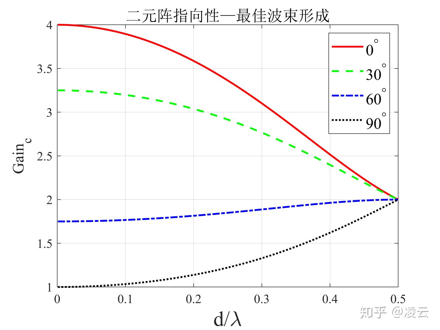
Figure 3(b)

Observing Figure 3(b), it can be found that when the best beamforming is used, when the beam viewing direction is the transverse direction ( $\ phi_o = 90 ^ \ circ$ ) $d / \ lambda$ , the directivity gradually decreases from 2 to 1 as it gradually decreases from 0.5 to 0. When the beam viewing direction is the end-fire direction ( $\ phi_o = 0 ^ \ circ$ ), with the $d / \ lambda$ gradual decrease from 0.5 to 0, the directivity gradually increases from 2 to 4, which is the super directivity.

The implementation code is as follows:

c = 340;
f = 1000;
lambda = c / f;
k = 2*pi*f/c; %波数
theta_angle=0:1:360;
theta=theta_angle*pi/180;
ratio_space = linspace(0.001, 0.5, 100);
space_list = ratio_space*lambda;  %连续阵间距
theta_d = [0 30 60 90] *pi/180;
color_list = {'r-' 'g--' 'b-.' 'k:'};
M = 2;
% 常规波束形成
figure;
for i = 1:length(theta_d)
   color = color_list{i};
   theta =  theta_d(i);
   Sinc = sin(k*space_list) ./ (k*space_list);
   Gain = 2 ./ (1+Sinc .* cos(k*space_list*cos(theta)));
   plot(ratio_space, Gain, color, 'linewidth', 1.5);
   hold on;
end
grid on;
xlabel('d/\lambda'); ylabel('Gain_c');
legend('0度', '30度', '60度', '90度', 'fontsize', 15);
title('二元阵指向性—常规波束形成');
% 最佳波束形成
figure;
for i = 1:length(theta_d)
   theta =  theta_d(i);
   color = color_list{i};
   Sinc = sin(k*space_list) ./ (k*space_list);
   Gain = (2 - 2*Sinc.*cos(k*space_list*cos(theta)))...
       ./ (1-Sinc.^2);
   plot(ratio_space, Gain, color, 'linewidth', 1.5);
   hold on;
end
grid on;
xlabel('d/\lambda'); ylabel('Gain_{opt}');
legend('0度', '30度', '60度', '90度', 'fontsize', 15);
title('二元阵指向性—最佳波束形成');

Reference books:

"Optimizing Array Signal Processing"

Binary array conventional beam pattern and its directivity—microphone array series (7)

Introduction to Binary Array

Guess you like