Support vector machines (SVM) are two classification algorithms. The so-called two classification is to divide data with multiple characteristics (attributes) into two categories. Among the current mainstream machine learning algorithms, neural networks and other machine learning models can already It is very useful to complete two classifications, multi-classifications, learning and research SVM, and understanding the rich algorithm knowledge behind SVM will be of great benefit to the future research of other algorithms; in the process of implementing SVM, the one-dimensional search, KKT conditions, and punishment introduced before will be comprehensively used Functions and other related knowledge. This article first explains the principle of SVM in detail, and then introduces how to use python to implement SVM algorithm from scratch.
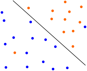
For ease of understanding, assuming that the sample has two attributes, the attribute values can be respectively mapped to the x and y axes of the two-dimensional space axis, as shown in the following figure:

The samples in the example are clearly divided into two categories. The black solid dots may be named category 1, and the hollow dots may be named category 2. In practical applications, the categories will be digitized. For example, category one is represented by 1, and category two is represented by -1. , And call the digitized category label. Each category corresponds to label 1, or -1 means that there is no hard and fast rule. You can do it according to your own preferences. It should be noted that since the SVM algorithm label also participates in mathematical operations, the category label cannot be set to 0 here.
It still corresponds to the above picture. If you can find a straight line, divide the above-mentioned solid point and hollow point into two parts. When there are other sample points next time, draw their attribute values as coordinates on the coordinate axis. The position relationship between the new sample point and the straight line can be used to determine its category. There are countless lines to satisfy such a line, SVM is to find the most suitable one: Observe the above picture, the green line is definitely not good, the classification line is already wrong without the verification set; and the blue line and red can be classified, blue The color line is too close to the solid black dot. In comparison, the red line is more'fair'. The red line is the classification straight line that SVM needs to find. The mathematical language to describe the "fairness" characteristic of the red line can be expressed as: treat the black point and the hollow point as two sets, if a straight line is found, some points in the black point set will be separated The straight line is the closest, and the distance from these points to the straight line is d; a series of points can be found in the hollow point set, the closest to the straight line, the distance is also d, then the straight line is what we want to find the linear classifier, and we call the two sets The point closest to the line is the support vector, and the SVM support vector machine is named after it.
Some algorithm books describe the SVM algorithm in this way to find a straight line that maximizes the space between the straight line and the closest point on both sides. It can also be seen from the figure above that the distance between the black point and the blue line is less than the distance to the red line (Right-angled hypotenuse). If you can find the support vector, you must find the classification line, and vice versa. The above is for two attribute values. By observing the two-dimensional plane, the characteristics of the SVM algorithm can be derived. If there are many sample attributes, how to summarize the regularity of the algorithm? First, let's talk about the separability theorem of lower convex sets. This theorem is not only the core theoretical support of SVM, but also the cornerstone of machine learning algorithms.
1. Convex set separability theorem
Let's take two-dimensional space as an example. In middle school, we learned straight line equations. For example, there is a straight line equation y=2x-1, as shown in the figure below:
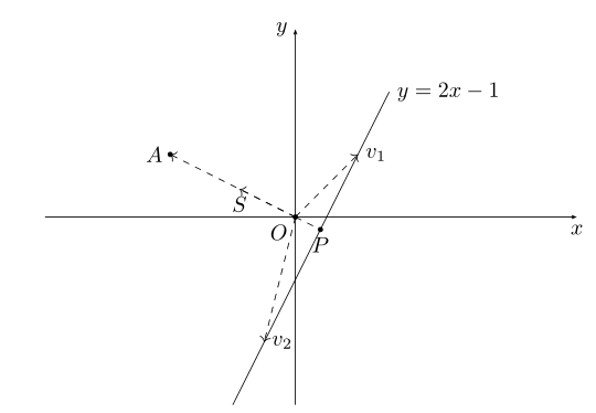
Write the linear equation y=2x-1 in inner product form:
Vector (-2,1) corresponding to the above figure the vector OA, the OA vector becomes a unit vector, i.e. the same direction OA, a vector mode is the OS, the coordinates S is  the same on both sides divided by the straight line equation
  can be obtained:
(x,y) represents any point on the straight line y=2x-1, the above formula shows that the inner product of any point on y=2x-1 and the unit vector S: is  , the length of the vector OP in the figure is
  , and the negative sign is because The direction of the OP vector is opposite to the direction of the OS; the vectors v1 and v2 in the above figure are all OP projected on the OS vector. This example shows: by introducing a vector OS, countless points on the line y=2x-1 can be on the vector OS used to represent, or that a straight line y = 2x-1 vector in the OS can use the coordinates (0, shown). Through the inner product projection method, high-dimensional data can be transformed into a real number on the vector. This is a linear functional process. In the field of mathematics, inner product is commonly used to reduce the data dimension, and the multi-dimensional data is processed into a real number for later analysis. deal with.
When extended to any dimension, the above equation can be expressed by a set formula: S:{x | pTx=α} x∈Rn. Corresponding to the above figure: the p vector corresponds to the vector OS, and x is any point on the line. In the SVM algorithm, the set S formed by the x points is called the hyperplane. Sometimes the inner product value of the high-dimensional data set projected to the vector p is a range: such as {x | pTx>=α} or {y | pTy<=-α}, the high-dimensional data is projected onto two intervals of the vector p :
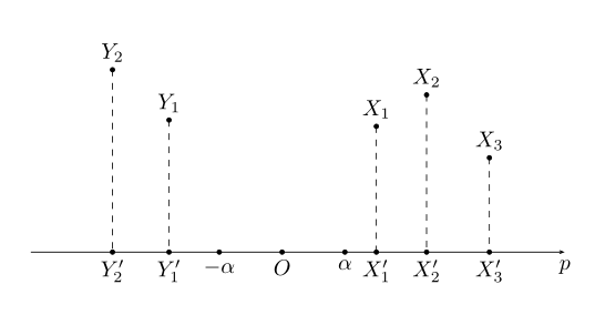
Next, introduce the convex set separation theorem:
In the above figure, X and Y are convex sets in the high-dimensional space, and X∩Y=Φ; after projecting X and Y onto the vector p, two convex sets X', Y'can be obtained, on the vector p X'and Y'must be at both ends of the vector p, that is, the two convex sets of X'and Y'are separable.
Note that there are two conditions in the theorem, one is that X and Y are convex sets, and the other is that the intersection of X and Y is an empty set. X', Y'separable means that the two can be distinguished on the vector p, and X and X', Y and Y'are all one-to-one mappings, X', Y'can be distinguished, which indirectly means X , Y can also be distinguished, the so-called'distinguishable' here is the dichotomy to be realized by SVM. The separability theorem of convex sets shows that two convex sets without intersection are linearly separable. At the same time, if the two data sets cannot be linearly separated, the data can be transformed into two convex sets by the kernel function, so the convex set separability theorem It also has a guiding significance for the generation of the kernel function.
Two, SVM algorithm
2.1 Hyperplane and maximum separation
As mentioned above, the linear classifier that can realize the two classification of data is called a hyperplane. The SVM algorithm needs to request the hyperplane with the largest interval. The hyperplane can be set as S:{x|pTx=α}, because pTx=α, etc. Both sides of the formula can be divided by a positive number to normalize p to a unit vector. It is better to set p to be a unit vector that has been processed. This setting does not affect the SVM algorithm. In general literature, hyperplanes are usually written in implicit function form:
S:{x|pTx-α=0} x∈Rn,p∈Rn,||p||=1
From the knowledge of geometry, the formula for the distance from any point x in the space to the hyperplane S is:
The distance between the support vectors belonging to the two categories and the hyperplane is d, d>0. Since the support vector is the closest point to the hyperplane in the respective classification data, the following inequality is available for all data:
 ⑴
⑴
Dividing both sides of formula (1) by d, we can get:,  using the exchange method, let:
 ⑵
⑵
This gives the common form of constraints:
 ⑶
⑶
Next, we need to remove the absolute value symbol from formula (3). SVM is a two-class classification problem: the classification label y=1 when ωTx+b>=1; the classification label y=- when ωTx+b<=-1 1. In this way, all data have inequalities:
y(ωTx+b)>=1 ④
Going back and looking at the exchange element setting, ω=pT/d, the norm operations on both sides of the equation are: ||ω||=||pT||/d=1/d, we can get d=1/| |ω||, the SVM algorithm needs to maximize the separation distance d on the basis of satisfying the constraints of formula 4. Assuming there are m data to be classified, implementing the SVM algorithm is equivalent to solving a nonlinear programming problem with inequality constraints:
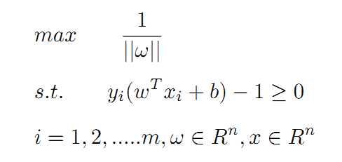
The above problem can also be expressed as a minimum problem:
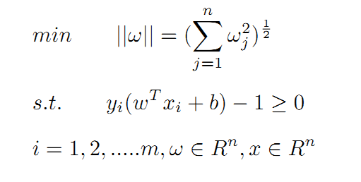 ⑤
⑤
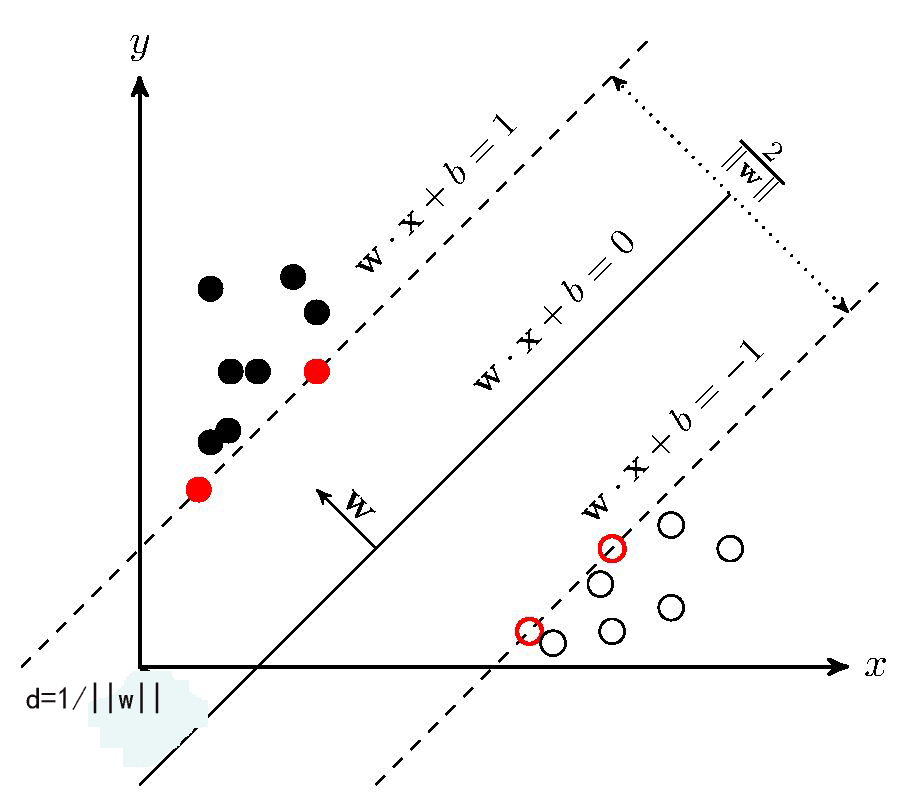
The classification effect of the hyperplane and the relationship between each parameter can be referred to the following figure:
2.2 Maximum soft interval
In practice, due to the existence of abnormal data, the hyperplane cannot completely divide the data into two parts, as shown in the figure below:
A small amount of abnormal data is mixed in the two classifications. Excluding a few abnormal points, the hyperplane in the above figure can separate most samples. The formula ⑤ can be compatible with the situation in the above figure after introducing slack variables:
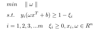 (5.1)
(5.1)
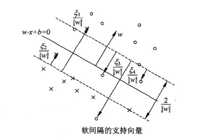
 Normally it is equal to 0, indicating that the sample points are listed on both sides of the support vector; >0 represents abnormal data : when 0 <<1, it represents the data is between the hyperplane and the support vector, as shown in the figure above 2 and point 4; and >1 means that the data is in the other side's space, such as point 1 and point 3 in the above figure. The interval that satisfies the formula (5.1) is called the soft interval. The optimization result of the soft interval not only requires the maximum interval of the support vector, but also makes each as small as possible . In other words , after the hyperplane is determined, the number of samples defined as abnormal data should be as small as possible.
[x_train, y_train, x_test, y_test]= data(); % load data

% Project part 1
disp('--------Project part 1----------');
plot_alldata(x_train, y_train, x_test, y_test); % plot all data
fit_data(x_train, y_train, x_test, y_test); % fitting data & plot the best model

% Project part 2
disp('--------Project part 2----------');
svm(x_train,y_train,x_test,y_test); % svm model fitting & plots
Result display
>> main_project
警告: 在为表创建变量名称之前,对文件中的列标题进行了修改,以使其成为有效的 MATLAB 标识符。原始列标题保存在 VariableDescriptions 属性
中。
将 'PreserveVariableNames' 设置为 true 以使用原始列标题作为表变量名称。
--------Project part 1----------
For n =
     1

mse_train=
   2.9834e+04

r2_train=
    0.1084

mse_test=
   3.2158e+04

r2_test=
    0.1305

---------------
For n =
     2

mse_train=
   1.3195e+04

r2_train=
    0.6057

mse_test=
   1.5085e+04

r2_test=
    0.6028

---------------
For n =
     3

mse_train=
   1.2732e+04

r2_train=
    0.6195

mse_test=
   1.4313e+04

r2_test=
    0.6237

---------------
For n =
     4

mse_train=
   1.2687e+04

r2_train=
    0.6208

mse_test=
   1.4152e+04

r2_test=
    0.6283

---------------
For n =
     5

mse_train=
   1.1969e+04

r2_train=
    0.6423

mse_test=
   1.3453e+04

r2_test=
    0.6470

---------------
For n =
     6

mse_train=
   6.3150e+03

r2_train=
    0.8113

mse_test=
   6.8526e+03

r2_test=
    0.8285

---------------
For n =
     7

警告: 多项式未正确设置条件。请添加具有不同 X 值的点,减少多项式的次数,或者尝试按照 HELP POLYFIT 中所述进行中心化和缩放。
> In polyfit (line 79)
  In fit_data (line 5)
  In main_project (line 6)
mse_train=
   6.2697e+03

r2_train=
    0.8126

mse_test=
   6.8162e+03

r2_test=
    0.8296

---------------
For n =
     8

警告: 多项式未正确设置条件。请添加具有不同 X 值的点,减少多项式的次数,或者尝试按照 HELP POLYFIT 中所述进行中心化和缩放。
> In polyfit (line 79)
  In fit_data (line 5)
  In main_project (line 6)
mse_train=
   3.0802e+03

r2_train=
    0.9079

mse_test=
   3.3461e+03

r2_test=
    0.9258

---------------
For n =
     9

警告: 多项式未正确设置条件。请添加具有不同 X 值的点,减少多项式的次数,或者尝试按照 HELP POLYFIT 中所述进行中心化和缩放。
> In polyfit (line 79)
  In fit_data (line 5)
  In main_project (line 6)
mse_train=
   2.9532e+03

r2_train=
    0.9117

mse_test=
   3.3297e+03

r2_test=
    0.9261

---------------
警告: 多项式未正确设置条件。请添加具有不同 X 值的点,减少多项式的次数,或者尝试按照 HELP POLYFIT 中所述进行中心化和缩放。
> In polyfit (line 79)
  In fit_data (line 32)
  In main_project (line 6)
model coefficient:
    0.0000   -0.0001    0.0074   -0.2230    3.8894  -39.3375  219.0309 -587.1015  589.8787    0.1253

--------Project part 2----------
-------Gaussian-------
CASE1 - default:
mse =
   1.4268e+03

r2 =
    0.9771

CASE2:
mse =
   1.6445e+03

r2 =
    0.9758

CASE3:
mse =
   1.4664e+03

r2 =
    0.9772

OPTIMIZED:
|====================================================================================================================|
| Iter | Eval   | Objective:  | Objective   | BestSoFar   | BestSoFar   | BoxConstraint|  KernelScale |      Epsilon |
|      | result | log(1+loss) | runtime     | (observed)  | (estim.)    |              |              |              |
|====================================================================================================================|
|    1 | Best   |      10.431 |     0.89758 |      10.431 |      10.431 |       394.32 |       736.91 |       10.115 |
|    2 | Accept |      10.437 |      0.1401 |      10.431 |      10.432 |    0.0011055 |     0.053194 |       47.555 |
|    3 | Best   |      10.426 |    0.071798 |      10.426 |      10.426 |       25.627 |       30.172 |        19150 |
|    4 | Accept |      10.426 |    0.054275 |      10.426 |      10.426 |       1.1377 |    0.0012314 |        14020 |
|    5 | Accept |      10.428 |     0.14271 |      10.426 |      10.426 |       470.09 |       836.88 |      0.41086 |
|    6 | Accept |      10.426 |    0.037576 |      10.426 |      10.426 |       2.6562 |    0.0010627 |       3310.4 |
|    7 | Accept |      10.426 |    0.034094 |      10.426 |      10.426 |    0.0010521 |       24.307 |       5816.8 |
|    8 | Best   |      10.074 |    0.065287 |      10.074 |      10.074 |       17.708 |     0.056046 |       1.6934 |
|    9 | Accept |      10.426 |    0.038535 |      10.074 |      10.074 |       132.62 |      0.08944 |       3956.1 |
|   10 | Best   |      9.9965 |     0.06095 |      9.9965 |      9.9965 |       21.302 |     0.036971 |      0.28347 |
|   11 | Best   |      8.3865 |     0.07324 |      8.3865 |      8.3867 |       642.83 |    0.0044812 |      0.22288 |
|   12 | Accept |      9.5704 |    0.046863 |      8.3865 |      8.3867 |       993.59 |    0.0028159 |       156.21 |
|   13 | Best   |      8.3864 |    0.071449 |      8.3864 |      8.3864 |       975.49 |    0.0012285 |      0.27834 |
|   14 | Accept |      8.3865 |    0.064198 |      8.3864 |      8.3862 |       507.99 |    0.0010299 |      0.24398 |
|   15 | Best   |      8.3853 |     0.06352 |      8.3853 |       8.386 |       611.28 |    0.0019797 |      0.51237 |
|   16 | Accept |      8.3865 |    0.069143 |      8.3853 |      8.3751 |       660.76 |    0.0013634 |      0.22497 |
|   17 | Accept |       8.386 |    0.068376 |      8.3853 |      8.3773 |       828.03 |    0.0024918 |      0.35096 |
|   18 | Accept |      8.3861 |    0.067393 |      8.3853 |      8.3799 |       732.96 |    0.0014109 |      0.32464 |
|   19 | Accept |      8.3861 |    0.062025 |      8.3853 |      8.3797 |       520.66 |    0.0022738 |      0.30965 |
|   20 | Accept |      8.3863 |    0.066882 |      8.3853 |      8.3797 |       668.85 |    0.0018481 |      0.24784 |
|====================================================================================================================|
| Iter | Eval   | Objective:  | Objective   | BestSoFar   | BestSoFar   | BoxConstraint|  KernelScale |      Epsilon |
|      | result | log(1+loss) | runtime     | (observed)  | (estim.)    |              |              |              |
|====================================================================================================================|
|   21 | Accept |      8.3866 |    0.063036 |      8.3853 |      8.3796 |       903.96 |    0.0023935 |      0.22712 |
|   22 | Accept |      8.3864 |    0.065384 |      8.3853 |      8.3807 |       988.43 |    0.0056305 |      0.26435 |
|   23 | Accept |      8.3857 |    0.080765 |      8.3853 |      8.3808 |       768.95 |    0.0028004 |      0.40427 |
|   24 | Accept |      10.434 |    0.047994 |      8.3853 |      8.3807 |     0.036485 |       962.56 |      0.22485 |
|   25 | Accept |      10.432 |    0.091279 |      8.3853 |      8.3805 |     0.065077 |     0.001002 |      0.22826 |
|   26 | Accept |      10.426 |     0.03629 |      8.3853 |      8.3804 |      0.15322 |       962.81 |        20662 |
|   27 | Accept |      8.3865 |    0.063816 |      8.3853 |      8.3815 |       648.08 |    0.0022537 |      0.24789 |
|   28 | Accept |      10.426 |    0.035603 |      8.3853 |      8.3814 |    0.0013648 |    0.0010192 |        21509 |
|   29 | Accept |      10.434 |    0.048371 |      8.3853 |      8.3813 |    0.0010406 |       767.16 |      0.32152 |
|   30 | Accept |      8.3866 |    0.079493 |      8.3853 |      8.3814 |       912.54 |    0.0035796 |      0.24067 |

__________________________________________________________
优化完成。
达到 MaxObjectiveEvaluations 30。
函数计算总次数: 30
总经过时间: 26.8651 秒。
总目标函数计算时间: 2.808

观测到的最佳可行点:
    BoxConstraint    KernelScale    Epsilon
    _____________    ___________    _______

       611.28         0.0019797     0.51237

观测到的目标函数值 = 8.3853
估计的目标函数值 = 8.3814
函数计算时间 = 0.06352

估计的最佳可行点(根据模型):
    BoxConstraint    KernelScale    Epsilon
    _____________    ___________    _______

       668.85         0.0018481     0.24784

估计的目标函数值 = 8.3814
估计的函数计算时间 = 0.067649

mse =
   2.0132e+03

r2 =
    0.9671

-------RBF-------
CASE1 - default:
mse =
   1.4268e+03

r2 =
    0.9771

CASE2:
mse =
   1.4664e+03

r2 =
    0.9772

CASE3:
mse =
   1.4591e+03

r2 =
    0.9766

OPTIMIZED:
|====================================================================================================================|
| Iter | Eval   | Objective:  | Objective   | BestSoFar   | BestSoFar   | BoxConstraint|  KernelScale |      Epsilon |
|      | result | log(1+loss) | runtime     | (observed)  | (estim.)    |              |              |              |
|====================================================================================================================|
|    1 | Best   |      10.437 |    0.064096 |      10.437 |      10.437 |    0.0024199 |     0.012131 |      0.82686 |
|    2 | Best   |      10.424 |    0.035964 |      10.424 |      10.425 |       792.75 |      0.51879 |       2798.3 |
|    3 | Accept |      10.424 |    0.033958 |      10.424 |      10.424 |    0.0015712 |       1.7285 |        12257 |
|    4 | Best   |      10.315 |    0.052699 |      10.315 |      10.315 |       64.709 |       60.677 |      0.43676 |
|    5 | Accept |       10.43 |    0.053824 |      10.315 |      10.341 |       598.05 |        816.9 |      0.22621 |
|    6 | Best   |      10.315 |    0.049229 |      10.315 |      10.315 |       65.348 |       60.686 |      0.73483 |
|    7 | Accept |      10.424 |    0.032769 |      10.315 |      10.315 |     0.068404 |       38.268 |       382.69 |
|    8 | Best   |       10.23 |    0.046858 |       10.23 |       10.23 |        163.2 |       61.687 |        38.56 |
|    9 | Accept |      10.424 |     0.03518 |       10.23 |       10.23 |       4.1446 |       62.152 |       2623.5 |
|   10 | Accept |      10.424 |    0.033162 |       10.23 |       10.23 |       199.56 |       62.459 |       2073.2 |
|   11 | Best   |      10.113 |    0.048122 |      10.113 |      10.113 |       307.74 |       60.662 |       18.094 |
|   12 | Accept |       10.44 |    0.052386 |      10.113 |      10.113 |    0.0020345 |       55.312 |       10.057 |
|   13 | Best   |      9.5718 |    0.048005 |      9.5718 |      10.002 |       694.03 |       28.973 |       12.634 |
|   14 | Best   |      7.8382 |    0.057983 |      7.8382 |      7.8399 |       932.32 |        4.265 |       11.006 |
|   15 | Accept |      10.433 |    0.041807 |      7.8382 |      7.8384 |      0.39209 |       4.3466 |       348.78 |
|   16 | Accept |       8.111 |    0.055765 |      7.8382 |      7.8388 |       976.56 |       5.5148 |       1.4862 |
|   17 | Accept |      10.424 |    0.032728 |      7.8382 |      7.8386 |       992.59 |       4.0578 |       2128.8 |
|   18 | Best   |        7.65 |    0.066125 |        7.65 |        7.65 |       819.88 |        2.352 |       4.6514 |
|   19 | Accept |      7.7333 |    0.062206 |        7.65 |      7.6576 |        912.6 |       3.2069 |       4.5506 |
|   20 | Best   |      7.6008 |    0.071054 |      7.6008 |      7.6011 |       990.85 |        1.656 |       8.9775 |
|====================================================================================================================|
| Iter | Eval   | Objective:  | Objective   | BestSoFar   | BestSoFar   | BoxConstraint|  KernelScale |      Epsilon |
|      | result | log(1+loss) | runtime     | (observed)  | (estim.)    |              |              |              |
|====================================================================================================================|
|   21 | Accept |      7.6387 |    0.098309 |      7.6008 |      7.6007 |       982.52 |      0.83259 |       2.7969 |
|   22 | Accept |      7.6275 |    0.076077 |      7.6008 |      7.6018 |       797.68 |       0.9112 |      0.29266 |
|   23 | Accept |      7.9363 |      0.0648 |      7.6008 |      7.6019 |       994.85 |      0.32932 |      0.23043 |
|   24 | Accept |      7.6935 |    0.045446 |      7.6008 |      7.6018 |       29.346 |        0.967 |      0.37377 |
|   25 | Accept |      7.6274 |    0.080696 |      7.6008 |      7.6017 |        910.2 |       0.9449 |      0.91925 |
|   26 | Accept |      7.6121 |    0.077758 |      7.6008 |       7.603 |          943 |       1.1589 |       5.0625 |
|   27 | Accept |      7.6153 |    0.062063 |      7.6008 |      7.6032 |       517.55 |       1.4588 |      0.25744 |
|   28 | Accept |      7.6051 |    0.058127 |      7.6008 |      7.6033 |       254.49 |        1.155 |      0.38512 |
|   29 | Accept |      7.6205 |    0.075103 |      7.6008 |       7.603 |       999.64 |       1.4418 |       1.9978 |
|   30 | Accept |      7.6088 |    0.051488 |      7.6008 |       7.604 |       227.74 |       1.2748 |       1.9489 |

__________________________________________________________
优化完成。
达到 MaxObjectiveEvaluations 30。
函数计算总次数: 30
总经过时间: 20.9975 秒。
总目标函数计算时间: 1.6638

观测到的最佳可行点:
    BoxConstraint    KernelScale    Epsilon
    _____________    ___________    _______

       990.85           1.656       8.9775

观测到的目标函数值 = 7.6008
估计的目标函数值 = 7.604
函数计算时间 = 0.071054

估计的最佳可行点(根据模型):
    BoxConstraint    KernelScale    Epsilon
    _____________    ___________    _______

       254.49           1.155       0.38512

估计的目标函数值 = 7.604
估计的函数计算时间 = 0.057088

mse =
   1.3855e+03

r2 =
    0.9748

-------Polynomial-------
CASE1 - default:
mse =
   1.6898e+04

r2 =
    0.6155

CASE2:
mse =
   1.5912e+04

r2 =
    0.6422

CASE3:
mse =
   6.6300e+03

r2 =
    0.8565

OPTIMIZED:
|====================================================================================================================|
| Iter | Eval   | Objective:  | Objective   | BestSoFar   | BestSoFar   | BoxConstraint|  KernelScale |      Epsilon |
|      | result | log(1+loss) | runtime     | (observed)  | (estim.)    |              |              |              |
|====================================================================================================================|
|    1 | Best   |      17.436 |      28.927 |      17.436 |      17.436 |       232.42 |     0.041278 |      0.77342 |
|    2 | Best   |       10.42 |    0.071368 |       10.42 |      10.775 |       21.908 |     0.010392 |        12625 |
|    3 | Accept |       10.42 |    0.043085 |       10.42 |       10.42 |    0.0058184 |       18.398 |       3455.5 |
|    4 | Accept |      71.286 |      28.847 |       10.42 |      11.828 |    0.0059341 |    0.0013698 |       2.1953 |
|    5 | Accept |       10.42 |    0.047948 |       10.42 |      10.418 |       24.457 |    0.0030582 |       9739.2 |
|    6 | Accept |       10.42 |    0.037128 |       10.42 |      10.418 |      0.10555 |       1.1212 |        22115 |
|    7 | Accept |      42.845 |      28.004 |       10.42 |      10.415 |       998.17 |    0.0026635 |       83.309 |
|    8 | Accept |       10.42 |    0.038793 |       10.42 |      10.412 |      0.36885 |    0.0012841 |       5198.9 |
|    9 | Accept |      81.729 |      28.321 |       10.42 |      10.418 |       944.81 |    0.0043766 |      0.22306 |
|   10 | Best   |       9.571 |     0.40222 |       9.571 |      9.5701 |       172.69 |      0.60399 |      0.77291 |
|   11 | Accept |      9.5906 |     0.17913 |       9.571 |      9.5705 |     0.021205 |      0.14439 |       154.14 |
|   12 | Accept |      10.435 |    0.045818 |       9.571 |      9.5705 |       42.148 |       256.32 |      0.22485 |
|   13 | Accept |       10.42 |    0.036242 |       9.571 |      9.5706 |       65.078 |       995.86 |       9943.1 |


Complete code or write on behalf of adding QQ1575304183