Let me make a statement first: The article is copied and pasted directly from the push in my personal official account. Therefore, friends who are interested in intelligent optimization algorithms can follow my personal official account: Heuristic Algorithm Discussion . I will share different intelligent optimization algorithms in the public account from time to time, classic ones, or new intelligent optimization algorithms proposed in recent years, with MATLAB codes attached.

"The algorithm shared today was only online on September 3, 2023. It has not been a week until today. It can be said to be one of the latest intelligent optimization algorithms, published on KBS~

I appreciate the source of inspiration for this algorithm, and find its mathematical modeling process more interesting. "

The Optical Microscope Algorithm (OMA) is inspired by the ability of optical microscopes to magnify target objects, using the naked eye for initial observation and simulating the magnification process through objective lenses and eyepieces. The performance of OMA was verified through two experiments. The algorithm is user-friendly and does not require initialization parameters: (1) OMA was compared with nine heuristic algorithms on 50 Benchmark functions, and the results showed that OMA performed better , The calculation time is shorter; (2) Apply OMA to solve engineering problems, including structure optimization and multi-resource balancing in multi-project scheduling. OMA not only shows superiority, but also uses the least number of evaluations of the objective function. The algorithm has the characteristics of good robustness, easy implementation, and few control parameters, and can be used to solve various numerical optimization problems. Its original reference is as follows:

“Cheng MY, Sholeh MN. Optical microscope algorithm: A new metaheuristic inspired by microscope magnification for solving engineering optimization problems[J]. Knowledge-Based Systems, 2023: 110939.”

01Source
of inspiration

I prefer the model inspiration for this algorithm. Next, I will talk about my understanding: When we use a microscope to observe objects, we need to adjust the objective lens and eyepiece to find an optimal observation effect. Then, this optimal observation effect corresponds to the optimal solution that the algorithm is looking for, and the process of debugging the objective lens and eyepiece corresponds to the iteration of the population, that is, the continuous debugging of the objective lens and eyepiece is equivalent to the continuous evolution of the population. Putting the object on the microscope stage corresponds to the population initialization of the algorithm. This abstract process is shown in Figure 1. The cyclic iteration of the algorithm is to constantly adjust the objective lens and eyepiece to find the optimal viewing angle.

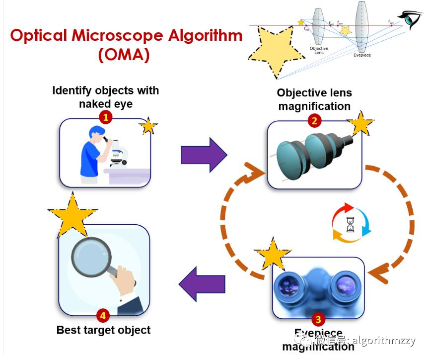
Figure 1 Algorithm framework of OMA

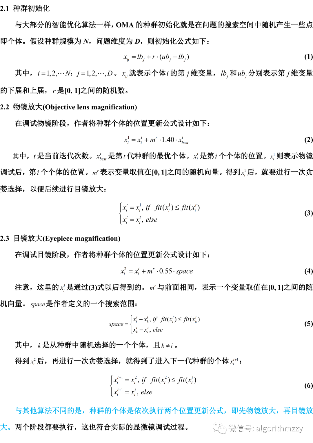
02Algorithm
design

As in previous posts, I will not edit mathematical formulas in the official account yet. Therefore, this part of the content is first written in the Word document, then made into a picture, and finally imported.

( To be honest, the design of OMA is quite simple, there are only two position update formulas, one corresponds to the objective lens magnification, and the other corresponds to the eyepiece magnification. )

03Calculation
process

The calculation flow chart of OMA is shown in Figure 2 (Note: Figure 2 is cut from the original text of GOA, so the meaning of the symbols in the figure needs to be compared with the original text):

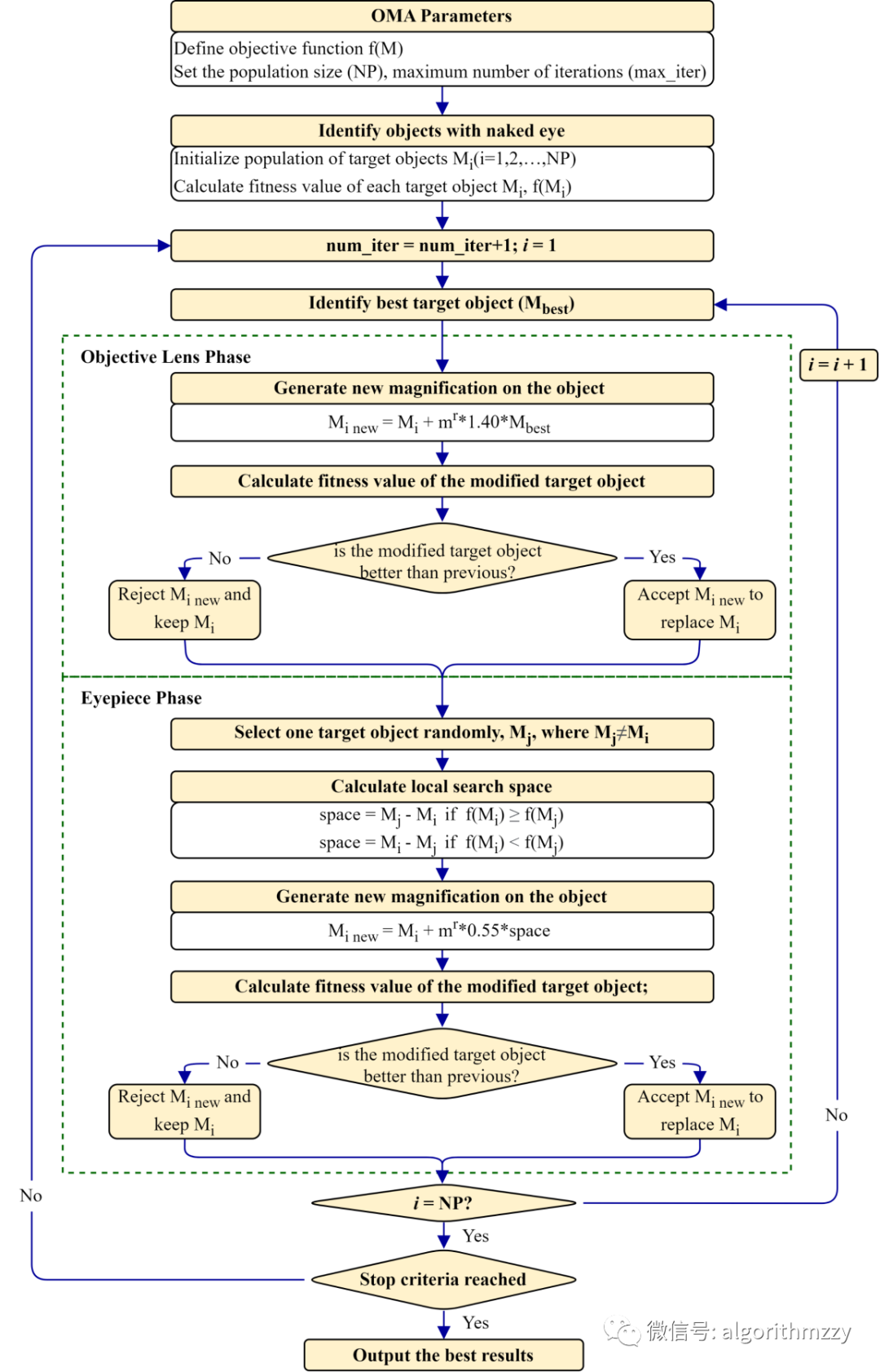
Figure 2 OMA calculation flow chart

04Experimental
Simulation

Here is a simple test of OMA performance. First, OMA is used for function optimization, and the MATLAB program of the algorithm is coded strictly according to its original reference. In addition, the population size is set to N equal to 50, and the Benchmark function uses the CEC2005 test set, CEC2013 test set, CEC2014 test set, CEC2017 test set, CEC2020 optimization function test set and CEC2022 optimization function test set respectively. The simulation results are briefly shown here without further analysis.

First, let’s test OMA’s ability to balance global exploration and local development. If you don’t know what I’m talking about, take a look at the previous push:
Exploration and Exploitation of the population (including MATLAB code),
as shown in Figure 3, which is the exploration and development of OMA on the CEC2005 test function f7. Development proportion curve.

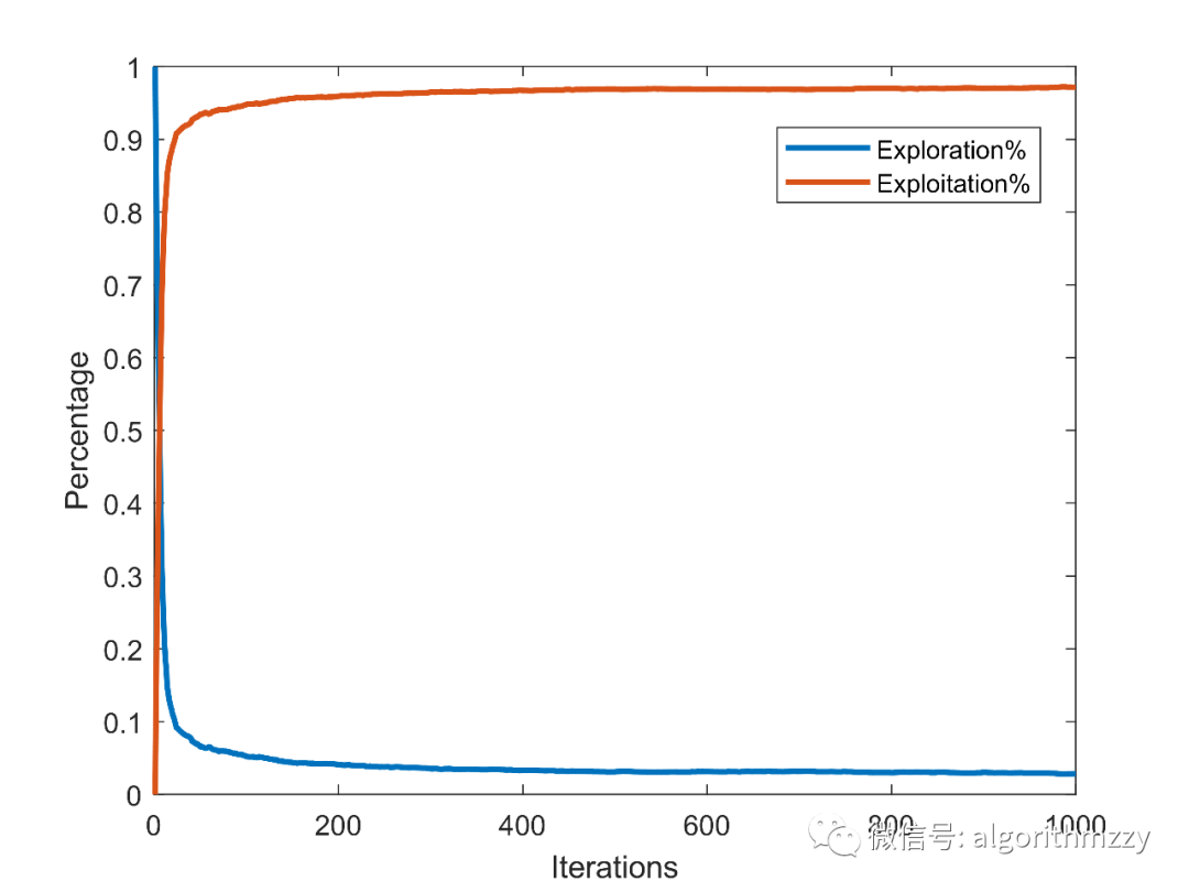
Fig. 2 The change curve of OMA's exploration and development percentage in CEC2005 f7

Secondly, taking the unimodal function Schwefel's 2.22 (f2) of CEC2005 as an example, the convergence effect of OMA in a 30-dimensional environment is demonstrated, as shown in Figure 4.

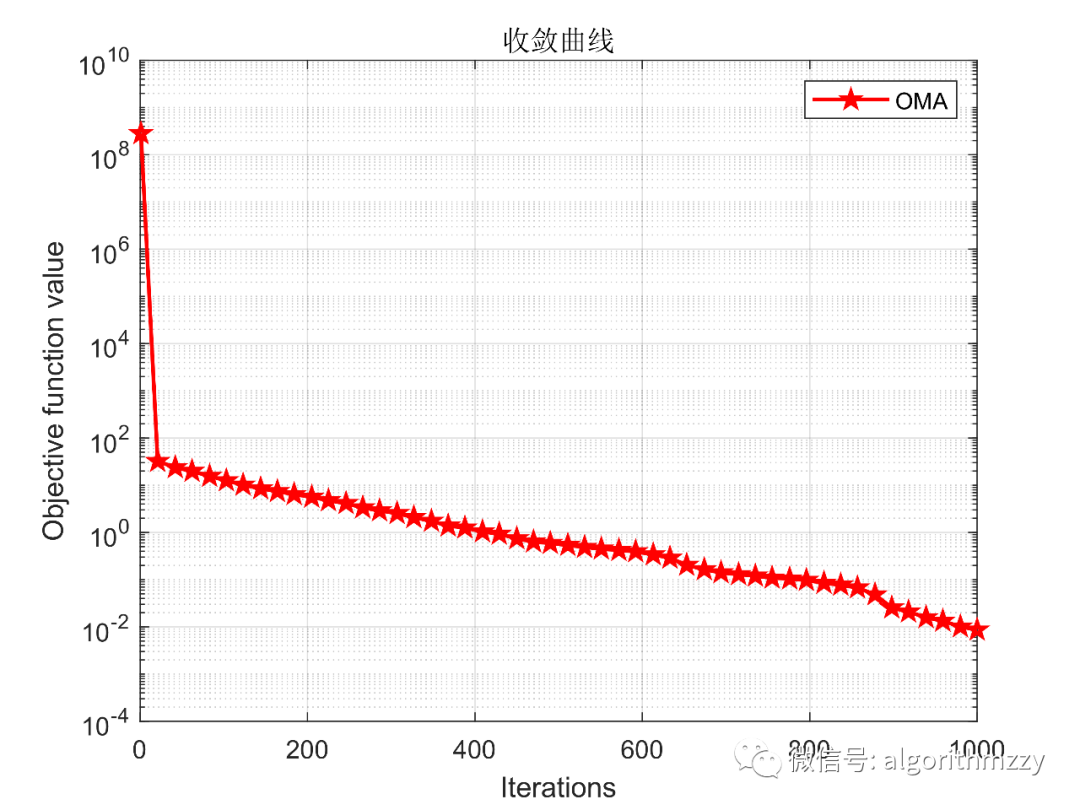
Figure 4 The convergence curve of OMA on the CEC2005 f2 test function

Again, taking the unimodal function F1 in the CEC2013 test set as an example to demonstrate the convergence effect of OMA in a 30-dimensional environment, as shown in Figure 5. (Note that the error curve is drawn)

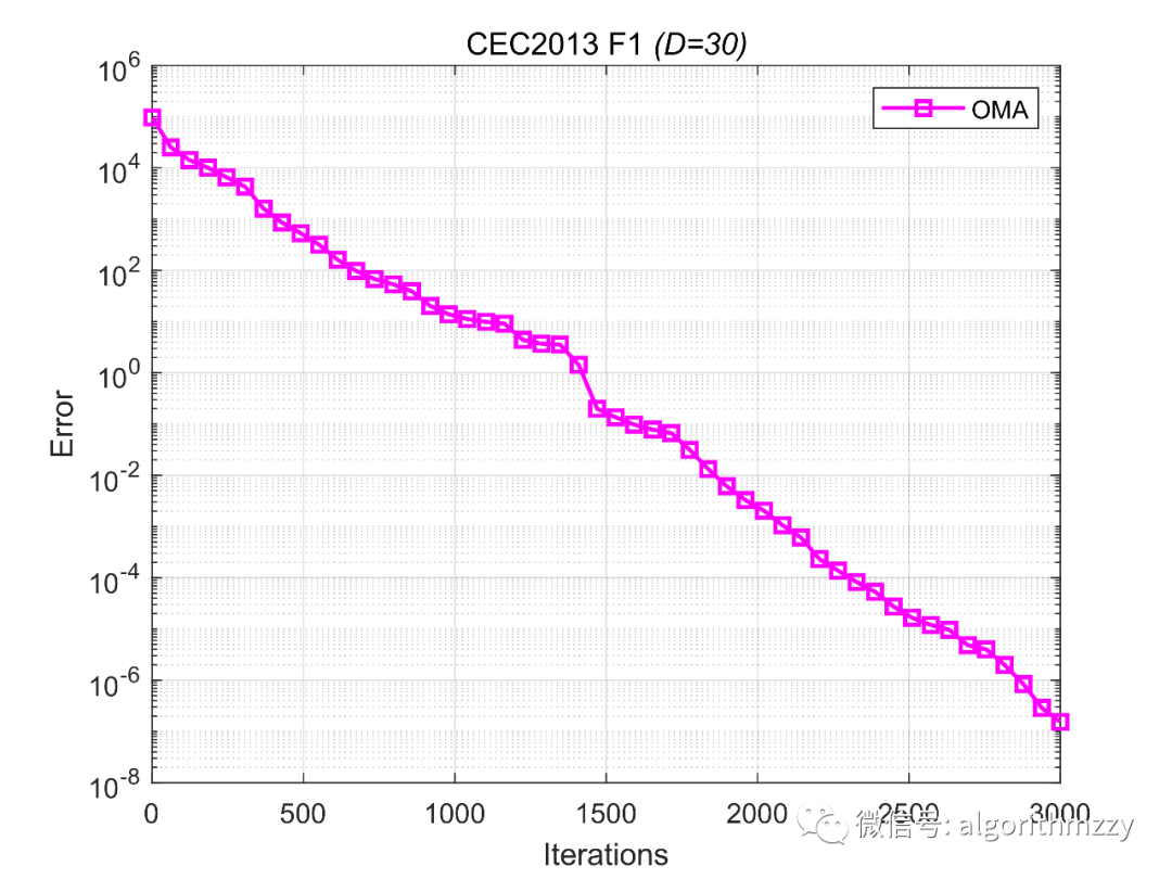
Figure 5 Error convergence curve of OMA on CEC2013 F1

Next, taking the multimodal function F14 in the CEC2014 test set as an example, the convergence effect of OMA in a 30-dimensional environment is demonstrated, as shown in Figure 6. (Note that the error curve is drawn)

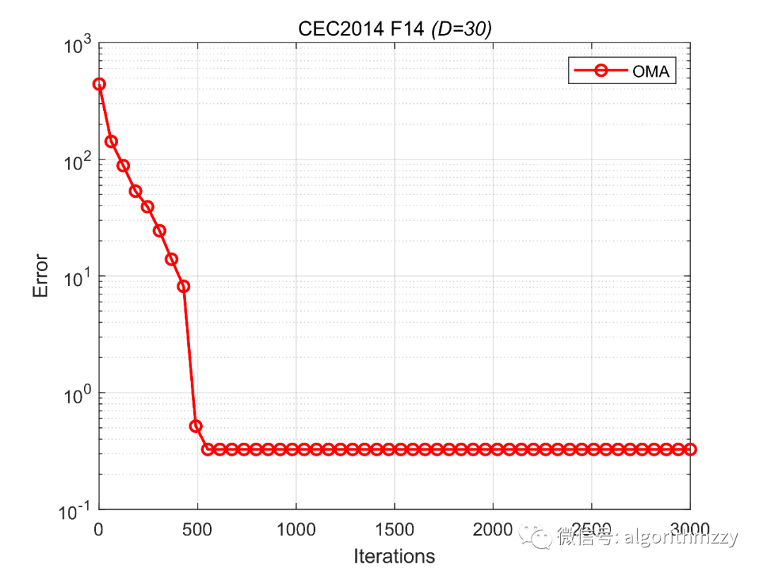
Figure 6 Error convergence curve of OMA on CEC2014 F14

Then, taking the multimodal function F4 in the CEC2017 test set as an example, we demonstrate the convergence effect of OMA in a 30-dimensional environment, as shown in Figure 7. (Note that the error curve is drawn)

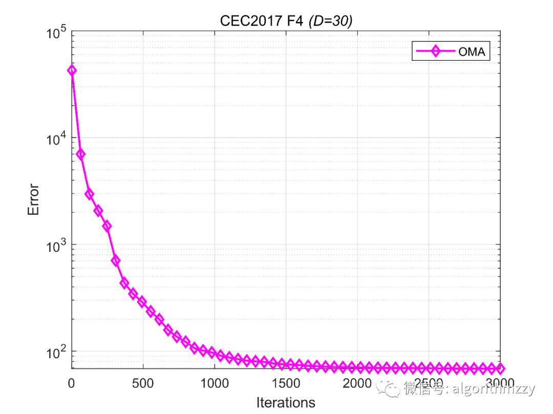
Figure 7 Error convergence curve of OMA on CEC2017 F4

After that, the unimodal function F2 in the CEC2020 optimization function test set is taken as an example to demonstrate the convergence effect of OMA in a 10-dimensional environment, as shown in Figure 8. (Note that the error curve is drawn)

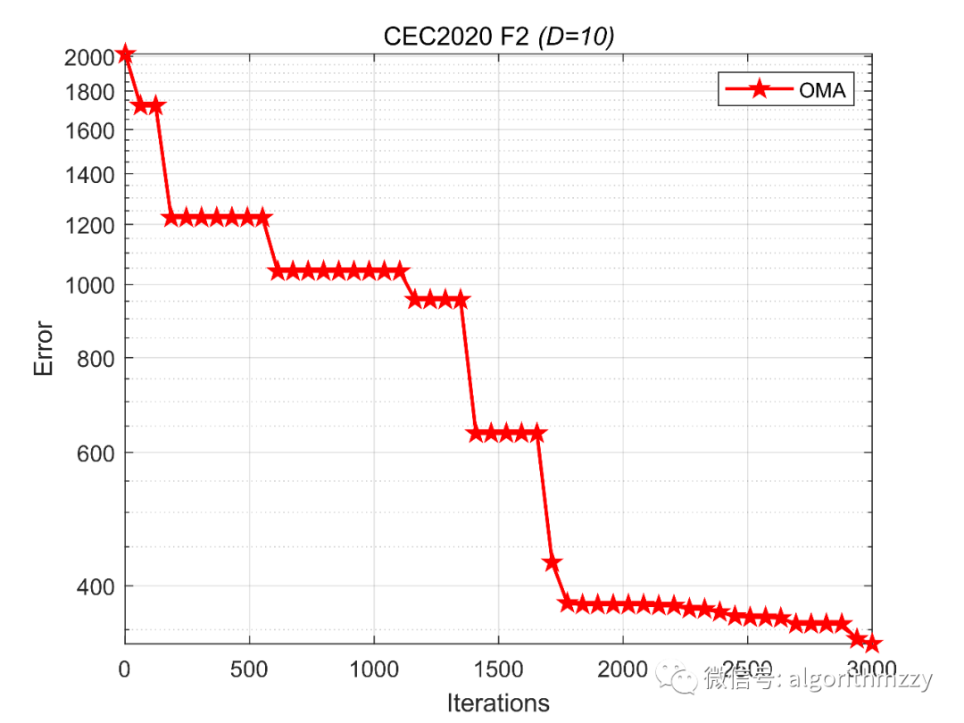
Figure 8 Error convergence curve of OMA on CEC2020 optimization function F2

Finally, the unimodal function F1 in the CEC2022 optimization function test set is taken as an example to demonstrate the convergence effect of OMA in a 10-dimensional environment, as shown in Figure 9. (Note that the error curve is drawn)

Figure 9 Error convergence curve of OMA on CEC2022 optimization function F1

Furthermore, OMA can be applied to complex engineering constrained optimization problems, such as the two-phase algorithm application content previously pushed:

Algorithm Application: Engineering Optimization Design Based on DBO Algorithm (Phase 1) (including MATLAB code)

Algorithm Application: Engineering Optimal Design (Phase 2) (including MATLAB code)

Here, the problem of pressure vessel design is taken as an example to show the solution effect of OMA. The convergence curve is shown in Figure 10.

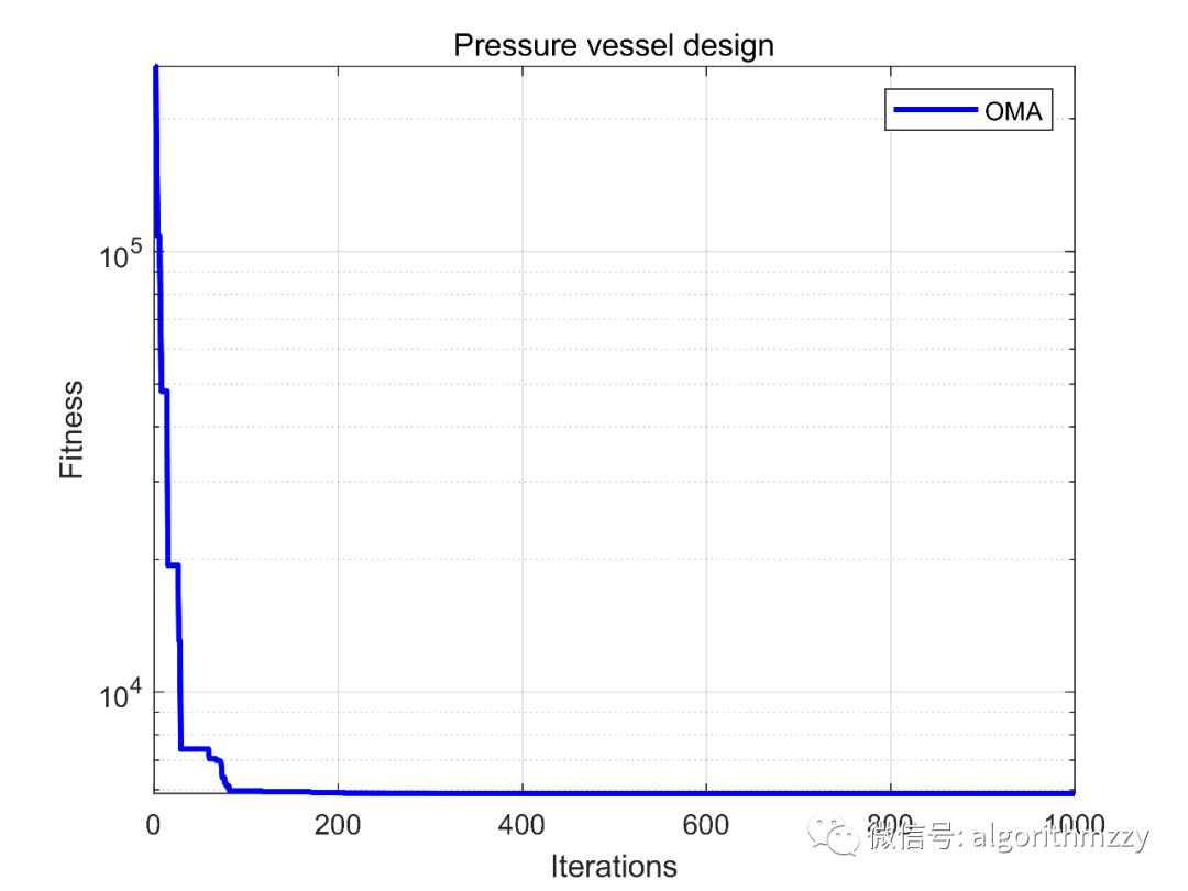
Fig.10 Convergence curve of objective function of OMA on pressure vessel design problem

Let me briefly talk about my opinion: the design of OMA is simple, the complexity is low, and the performance is quite satisfactory. I tried it, and the performance on engineering optimization problems is not bad. There are two suggestions:

1.OMA can be selected as the comparison algorithm. It is a new algorithm just published, and it is an article on KBS, where the journal level is placed. However, the performance of OMA is not very good, and it may be better to improve its own algorithm appropriately.

2. OMA can also be used as an improved algorithm. It is very new and its performance is quite satisfactory, so there are many things that can be improved, unlike some algorithms that cannot be changed. You can try to apply the improvement strategies of other algorithms to OMA to see the effect. In addition, I think the source of inspiration for OMA is quite novel. The constants in it are all taken from the actual values on the microscope equipment. The design is quite reasonable and not forced. So you can try to do some work.

05
MATLAB code

OMA runs CEC2005 test set