
Author: Yu Fan
background
Complex space-time systems modeled by partial differential equations are ubiquitous in many disciplines, such as applied mathematics, physics, biology, chemistry, and engineering. In most cases, we are unable to obtain analytical solutions to PDEs used to describe these complex physical systems, so numerical solution methods have been extensively studied, including: finite element, finite difference, isogeometric analysis (IGA) and other methods . Although these traditional numerical methods can well approximate the exact solution of the equation through basis functions, there is still a huge computational overhead in data assimilation and solving the inverse problem.
In recent years, various deep learning methods have emerged in an endless stream to solve forward and inverse problems of nonlinear systems. Research on using DNN to model physical systems can be roughly divided into the following two categories: continuous networks and discrete networks. A typical representative of continuous networks is PINNs: the residual of PDE is used as a soft constraint of the neural network, and a fully connected layer is used to approximate the solution of the equation, and the model can be performed on small data scale or even unlabeled sampled data. train. Nonetheless, PINNs are often limited to low-dimensional parameterizations and are stretched when facing PDE systems with steep gradients and complex local morphologies. Recently, a small number of pilot studies have found that discrete networks have better scalability and faster convergence speed than continuous learning. For example, CNN can be used as a proxy model in the rectangular domain for time-independent systems; PhyGeoNet uses physical and reference domains. To geometrically adaptively solve steady-state partial differential equations through coordinate transformation, for time-dependent systems, most neural network solution methods are still based on data-driven and meshing.
PhyCRNet[1], proposed by Professor Sun Hao's team at Renmin University of China's Hillhouse School of Artificial Intelligence, in collaboration with Northeastern University (USA) and the University of Notre Dame, is an unsupervised method for solving PDEs in multi-dimensional spatiotemporal domains through physical prior knowledge and convolutional recursive network architecture. Learning method, which combines ConvLSTM (extracting low-dimensional spatial features and learning time evolution), global residual connection (strictly mapping changes in equation solutions on the time axis) and high-order finite difference spatiotemporal filtering (determining the construction of a residual loss function The ability of the required PDE derivatives) makes it a basic solution when facing inverse problems and when there are sparse and noisy data.
1. Problem definition
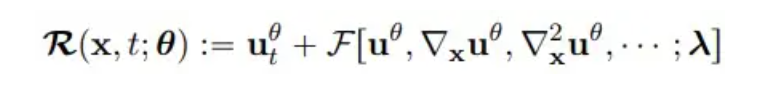
Considering multidimensional nonlinear parametric partial differential equations, the general form is as follows:
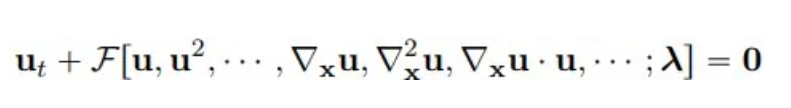
where u(x, t) represents the solution of the equation in the time domain T and the space domain Ω, and F is a nonlinear functional with parameter λ.
**2. ** Model method
ConvLSTM
ConvLSTM is a spatiotemporal sequence-to-sequence learning framework that extends from LSTM and its variant LSTM encoder-decoder prediction architecture (which have the advantage of modeling long-period dependencies that evolve over time). In essence, the memory unit is updated with the input and state information being accessed, and the accumulation and clearing of memory is completed through cleverly designed control gates. Based on this setting, the gradient disappearance problem of ordinary recurrent neural networks (RNN) is alleviated. ConvLSTM inherits the basic structure of LSTM (i.e., cell units and gates) to control information flow, and modifies the fully connected neural network (FC-NN) to take into account that CNN has better spatial connection representation capabilities and perform gating operations on CNN. As a special type of RNN, LSTM can be used as an implicit numerical method to solve time-dependent PDE equations. The structure diagram of a single ConvLSTM unit is as follows:
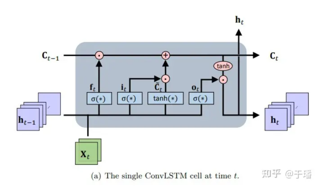 Figure 1: Single ConvLSTM cell at time t
The mathematical representation of updating a ConvLSTM unit is as follows:
Among them, * represents the convolution operation, ⊙ represents the Hadamard product; W is the weight parameter of the filter, and b represents the bias vector.
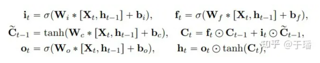
Pixel Shuffle
Pixel Shuffle is an efficient sub-pixel convolution operation that upsamples a low-resolution (LR) image to a high-resolution (HR) image. Assume that the dimensions of an LR feature tensor are (C An HR tensor with dimensions (C, H xr, W xr).  Figure 2: Pixel Shuffle layer
The efficiency of Pixel Shuffle is reflected in: (1) only increasing the resolution in the last layer of convolution, which can avoid the need to use more convolution layers to increase the image to the target resolution such as deconvolution; (2) ) In all feature extraction layers before the upsampling layer, smaller filters can be used to process these low-resolution tensors.
PhyCRNet
PhyCRNet consists of encoder-decoder modules, residual connections, autoregressive processes, and a filter-based differential method. The encoder contains three convolutional layers to learn low-dimensional latent features from the state variable Ui at a certain moment, and let it evolve over time through ConvLSTM. Since the transformation is performed on low-dimensional variables, the memory overhead will be reduced accordingly. In addition, inspired by the forward Euler method, we can add a global residual connection between the input variable Ui and the output variable Ui+1, and the single-step learning process can be expressed as Ui+1 = Ui + δt x N[Ui; θ], where N[·] represents the trained neural network operator, and δt is the unit time interval. Therefore, this recursive relationship can be viewed as a simple autoregressive process.
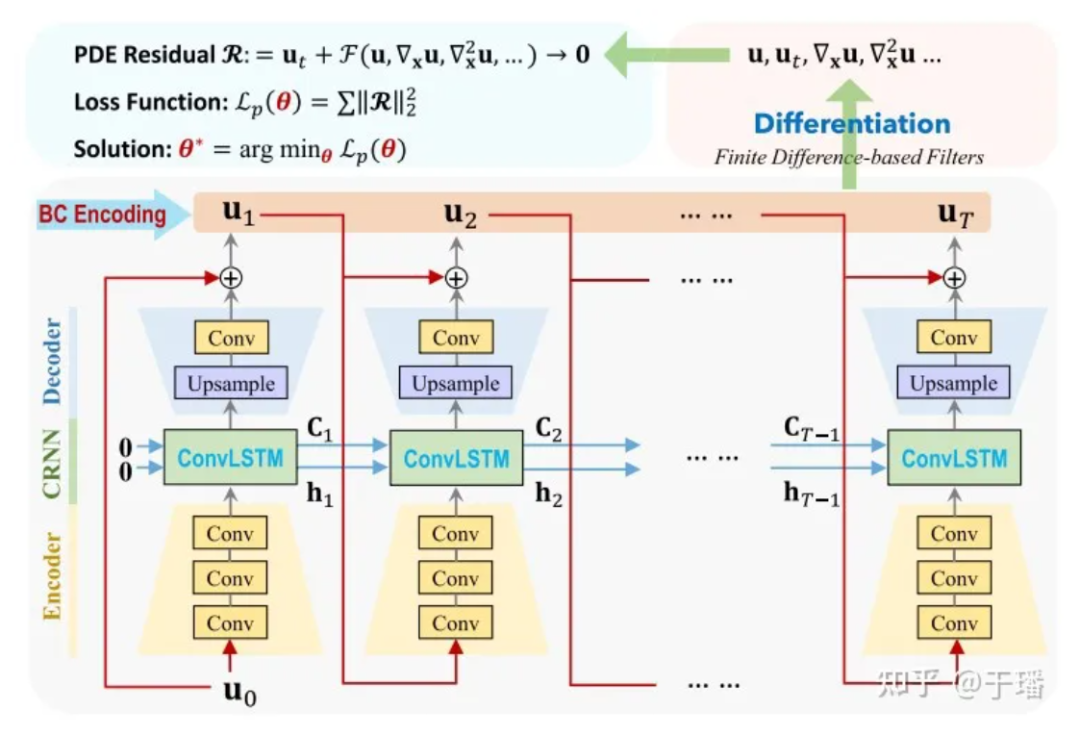 Figure 3: PhyCRNet network structure diagram
Here U0 is the initial condition, U1 to UT are the discrete solutions that need to be predicted by the model, and the time evolution from input to output. Compared with traditional numerical methods, ConvLSTM can use a larger time interval. For the calculation of each differential term, we use a fixed convolution kernel [1] to represent their difference values. In PhyCRNet, second-order and fourth-order difference terms are used to calculate the derivatives of U with respect to time and space. In order to further optimize computing performance, we can skip the encoder part in a cycle of size T, except for the first moment of each cycle. The schematic diagram is as follows:
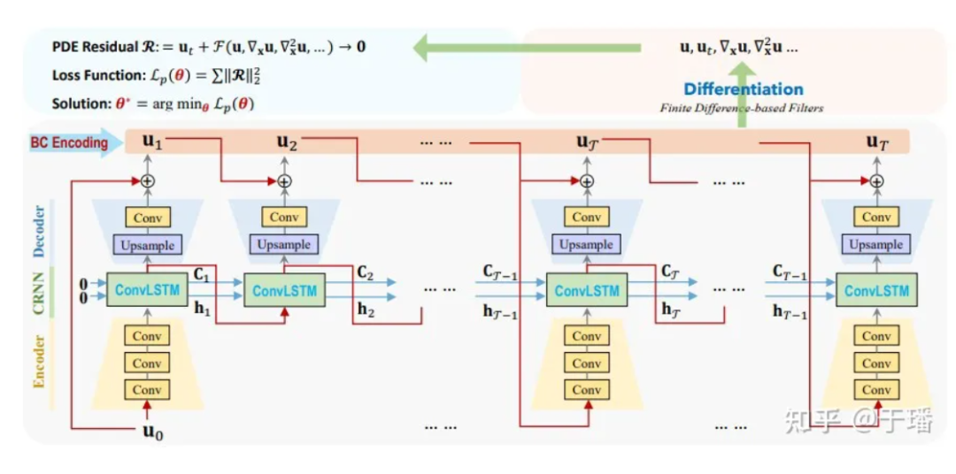 Figure 4: PhyCRNet-s network structure diagram
I/BC hard constraints
Compared with the PINNs method, which uses physical initial boundary conditions as soft constraints (its residuals are optimized as part of Loss), PhyCRNet uses the method of hard-coding I/BC into the model (the initial conditions are used as the input U0 of ConvLSTM, and the boundary Conditions are encoded through padding), so that physical conditions are no longer a soft constraint, thereby improving the accuracy and convergence speed of the model. For Dirichlet BC, the known constant boundary values can be filled directly as padding in the space domain; while for Neumann BC, a layer of ghost elements can be added around the space domain. (ghost elements), their values are approximated by differences during the training process.
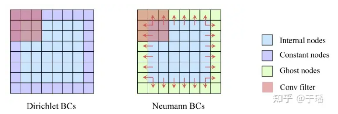 Figure 5: Illustration of hard constraints on boundary conditions
loss function
Since I/BC has been rigidly constrained in the model, the loss function only needs to include the residual term of the PDE. Taking a two-dimensional PDE system as an example, the loss function can be expressed as:
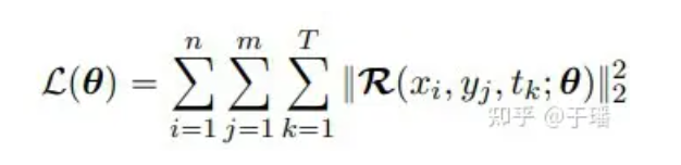
where n and m represent the height and width of the grid, T is the total number of time steps, and R(x, t; θ) is the residual of PDE:
**3. ** Result analysis
To evaluate the model error in the entire domain, the cumulative root mean square error (a-RMSE) at time τ is calculated as follows:
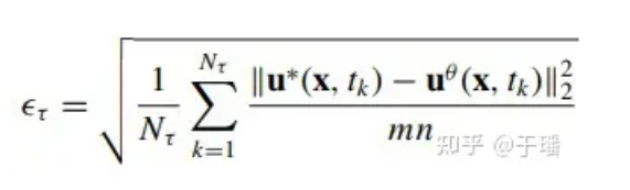
where Nτ is the number of time steps in [0, τ], and u*(x, t) is the reference solution of the equation.
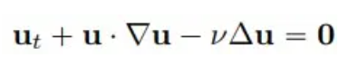
Two-dimensional Burgers equation
Consider a classic problem in fluid mechanics, given the two-dimensional Burgers equation of the following form:
We select 4 time points: training (t = 1.0, 2.0) and extrapolation (t = 3.0, 4.0) to compare the solution accuracy and extrapolation capabilities of PhyCRNet and PINN methods:
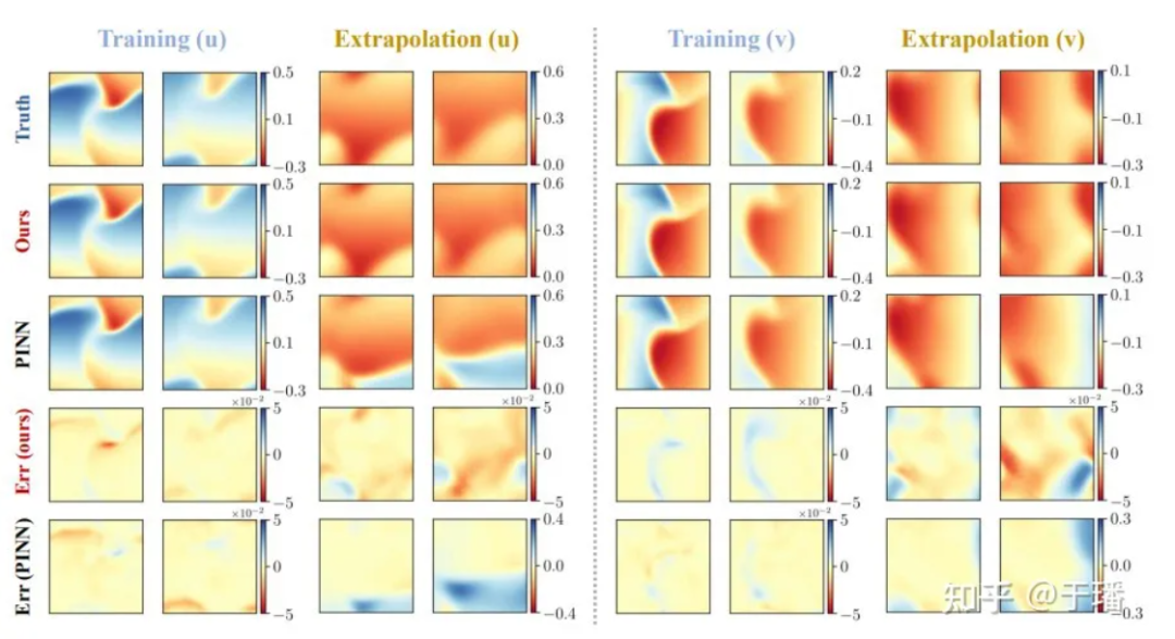 Figure 6: Training and extrapolation results of PhyCRNet versus PINNs for the two-dimensional Burgers equation
λ-ω RD equation
As a second case, consider a two-dimensional λ-ω RD system (often used to represent multi-scale biochemical processes):
Among them, u and v are two field variables that satisfy:
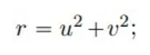
λ and ω are two real-valued functions:
The reference solution for a total of 801 time steps in the area [-10, 10] is generated by the spectral method; after training for 200 time steps in the [0, 5] time period, the reference solution for [5, 10] Prediction is made during the period, and the prediction results comparing PhyCRNet and PINN are as follows:
 Figure 7: PhyCRNet vs. PINNs training and extrapolation results for the λ-ω RD equation
The figure below shows the error propagation curves of PhyCRNet and PINNs during training and extrapolation in the two PDE systems mentioned above. It can be clearly seen that PhyCRNet performs better in both stages (especially the extrapolation stage).
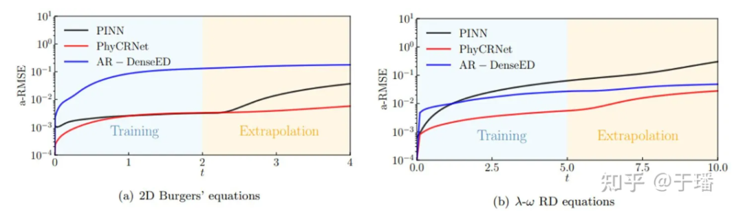 Figure 8: Comparing error propagation of PhyCRNet and PINNs
references
[1] Ren P, Rao C, Liu Y, et al. PhyCRNet: Physics-informed convolutional-recurrent network for solving spatiotemporal PDEs[J]. Computer Methods in Applied Mechanics and Engineering, 2022, 389: 114399.
[2]https://www.sciencedirect.com/science/article/abs/pii/S0045782521006514?via%3Dihub
A programmer born in the 1990s developed a video porting software and made over 7 million in less than a year. The ending was very punishing! Google confirmed layoffs, involving the "35-year-old curse" of Chinese coders in the Flutter, Dart and Python teams . Daily | Microsoft is running against Chrome; a lucky toy for impotent middle-aged people; the mysterious AI capability is too strong and is suspected of GPT-4.5; Tongyi Qianwen open source 8 models Arc Browser for Windows 1.0 in 3 months officially GA Windows 10 market share reaches 70%, Windows 11 GitHub continues to decline. GitHub releases AI native development tool GitHub Copilot Workspace JAVA is the only strong type query that can handle OLTP+OLAP. This is the best ORM. We meet each other too late.