Essay Lecture | Quantum Computing Two-Dimensional Isometric Tensor Network State

The open source China community team made its first live broadcast, telling the story behind the open source China community in the name of sharing."

Sharer: Wu Shaojun ｜School**: University of Electronic Science and Technology of China**

brief introduction

Overcoming the exponential growth in complexity when simulating quantum many-body systems is a challenging goal in physics. Currently, for the ground state properties of one-dimensional quantum systems, methods based on tensor network states (TNS) have provided an effective way to give basically accurate numerical solutions. In two-dimensional systems, some progress has also been made by introducing some algorithms to optimize TNS for various lattice models. This time, we will introduce a new quantum state representation method, namely Isometric TNS, which can be used to describe the quantum state of a two-dimensional system and has computational advantages. In addition, we will also introduce how to use local measurements to reconstruct the quantum state. A method to construct MPS, which has only a linear number of operations.

Related papers 1

**Title: Isometric Tensor Network States in Two Dimensions
Author: Michael P. Zaletel and Frank Pollmann
Journal: **Phys. Rev. Lett. 124, 037201 (2020)

**Published date:** January 24, 2020

Related Papers 2

**Credit: Efficient quantum state tomography
Credits: Marcus Cramer, Martin B. Plenio, Steven T. Flammia, Rolando Somma, David Gross, Stephen D. Bartlett, Olivier Landon-Cardinal, David Poulin & Yi-Kai Liu
:** Nature Communications 1, 149(2010)

**Published:** December 21, 2010

** introduction
**

(Image source: Nature volume 618, pages500–505 (2023))

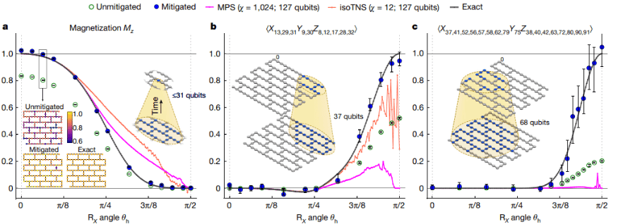
Recently, IBM implemented the simulation of the 2-dimensional transverse field Ising model on 127 quantum processors. For comparison, classical simulations need to be used to obtain accurate results. This work uses weight-1, weight-10 and weight-17 observations to measure the 5-step trotter's quantum circuit, and the experimental results are shown in the figure.

When performing classic simulations in order to obtain accurate solutions, the Light-cone and depth-reduced (LCDR) method is used here. It is divided into two parts. One part is to reduce the number of circuit layers that need to be simulated through the characteristics between quantum gates; the other part is to consider that the qubits related to the observation quantity A are local, which means that only a part of the qubits need to be considered. Evolution can then calculate the result of the final observation instead of all 127 bits. The related qubit numbers of weight-1, weight-10 and weight-17 observations are 31, 37 and 68 respectively. It is worth noting that the simulation with 68 qubits is still beyond the capabilities of brute force simulations by classical computers. Therefore, this work introduces tensor networks, 1D matrix product states (MPS) and 2D isometric tensor network states (iso TNS), for simulation.

** Introduction to Matrix Product State (MPS)
**

1. Basic knowledge of tensors

(1) Definition and graphical representation

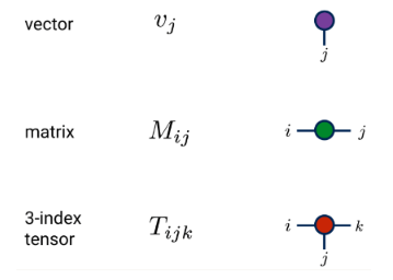
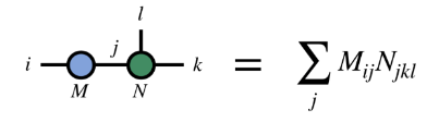
(2) Shrinkage of the same indicator

2、MPS

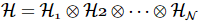
For a one-dimensional system with N grid points, if each grid point has d quantum states, the multi-body Hilbert space can be expressed as the tensor product of the grid Hilbert space:

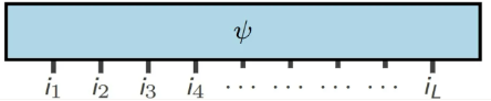
The corresponding arbitrary multiple postures can be expressed as:

(Image source: arXir:1603.03039, 2016)

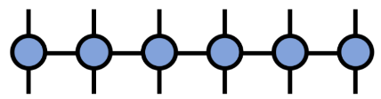
The core idea of matrix product state (MPS) is to express the multi-body state as:

(Image source: arXir:1603.03039, 2016)

Each unit is a third-order tensor, in which the physical index is the grid point quantum state, and the auxiliary index can be regarded as the quantum entanglement between it and the left and right systems.

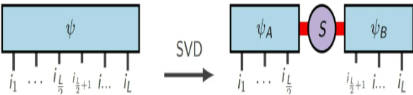
SVD decomposition:

For a general complex matrix A, there is a decomposition such that , where

is a diagonal matrix with dimension , and the elements on the diagonal are called singular values. Generally speaking, singular values are arranged in order from largest to smallest along the diagonal.

(Image source: arXir:1603.03039, 2016)

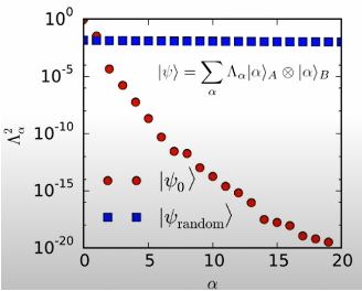
Where S represents singular value. If the entanglement between the two parts of the system is not strong, the spectrum of singular values tends to decay quickly, and only fewer singular values need to be retained to retain most of the information of the matrix. Suppose we stipulate that each group of Schmidt decompositions retains no more than m singular values. In the end, we only need a real number to approximately represent this multi-body state. Compared with the original representation method that requires 1 parameter, this representation has a linear space complexity for the number of grid points, and the efficiency is much higher than the exponential growth complexity of the original tensor product representation.

(Image source: arXir:1603.03039, 2016)

The process of getting MPS:

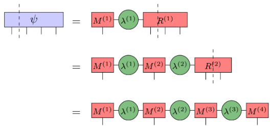
(Image source: arXir:1603.03039, 2016)

BECAUSE:

For a many-body operator, like states, we can write the many-body operator in matrix product form (MPO):

Different from states, the Hamiltonian composed of local operators can naturally be written in the form of matrix products:

(Image source: arXir:1603.03039, 2016)

The matrix product operator still maintains the matrix product structure after acting on the matrix product state:

(Image source: arXir:1603.03039, 2016)

Isometric tensor network states in two dimensions

1. Abstract

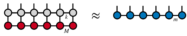
Tensor network states are a promising but numerically challenging tool for two-dimensional quantum many-body problems. In this article, the authors introduce isometrically restricted TNS ansatz, a form that allows efficient shrinkage of tensor networks. In order to numerically benchmark ansatz, the authors first demonstrated that the MPS representation of the ground state of the two-dimensional transverse field Ising model can be effectively converted to isoTNS. In fact, the authors implemented a 2D TEBD algorithm and showed that it effectively finds the isoTNS form. Approximation of the ground state of the 2D model.

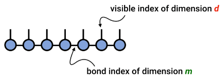
2. Isometric tensor network state

1) Isometry condition: for a dimensional matrix M, or

. In tensor diagrams, arrows are generally used to indicate orthogonality, which stipulates that the unit matrix is obtained by shrinking the inward index of the tensor and its conjugate tensor.

2) Canonical form of MPS:

Among them, A and B satisfy the left and right orthogonal conditions. The left orthogonal condition means that the contraction of the previous quantum and its own transposition is a unit matrix, and the right orthogonal condition means that the contraction of the following quantum and its own transposition is a unit matrix, representing a diagonal element. The decreasing diagonal matrix is also called the orthogonal center.

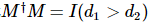
3) The expected value of the local operation can be directly 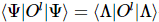obtained by, because its external AB tensor shrinks to 1 according to the isometry condition.

(Image source: Phys. Rev. Lett. 124, 037201)

Generalize to two dimensions:

By analogy with the above formula, we require that each row and column of TNS be an isometry. This constraint can be further required by requiring each tensor to be an isometry. As shown in Figure d above, the red part only has inward arrows. Therefore, this is the one-dimensional "orthogonal hypersurface" of TNS, which is the wave function under the standard orthonormal basis. Therefore, it can be processed like MPS and can be itself put into a one-dimensional canonical form (its orthogonal center can be moved freely using the one-dimensional canonical algorithm). For any operator , there is , that is, there is a dimensionality reduction of the one-dimensional expected value that can be efficiently computed by the standard MPS algorithm without further approximation. This is in sharp contrast to general TNS, where the expected value requires using an approximate shrinkage of the entire network.

3. Moving orthogonal hypersurface

The central orthogonal form is only computationally useful if the orthogonal hypersurface Lammda can be moved efficiently throughout the network. In one dimension, we can achieve the movement of the orthogonal center through the decomposition (QR or SVD) of any orthogonal matrix. In two dimensions, we also need to move the entire column. But for two-dimensional systems, the method of orthogonal matrix decomposition is invalid because it destroys the locality required to be expressed as an MPS.

(Image source: Phys. Rev. Lett. 124, 037201)

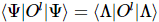
In this article, the author uses the Moses Move method to move the center of the orthogonal surface. As shown in the figure above, after the MM algorithm, the orthogonal hypersurface is divided into the product of left orthogonal and zero column states without physical indicators . Among them, decompression is accomplished by continuously applying the "splitting" process shown in Figure (b). The index of the center point is grouped into three states and "split" into three tensors in two steps.

4. MPS extended to isoNTS

(Image source: Phys. Rev. Lett. 124, 037201)

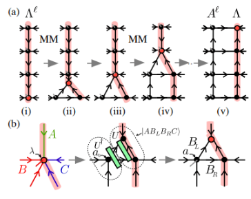
Given a ground-state wave function , the authors proposed an iterative algorithm that can be put into isoTNS and tested the sing transverse field model. Consider a strip and use DMRG to obtain the ground state of a 1D MPS, where each "site" contains the corresponding row of spins [Figure (a)]. As shown in the 3rd panel in Figure a, MM can then be used to iteratively "split" the columns of the wave function 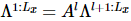, producing isoTNS. In this example, the bond dimension is selected as 6. When g=3.5 (paramagnetic phase), the error at each site is . In this case, . The results are shown in Figure b, which shows that the entanglement entropy of segmentation along the orthogonal hypersurface decreases as the number of iterations increases. Figure c illustrates that as the number of iterations increases, the entanglement entropy decays linearly, which is in line with expectations.

5. Algorithm

(Image source: Phys. Rev. Lett. 124, 037201)

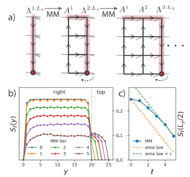
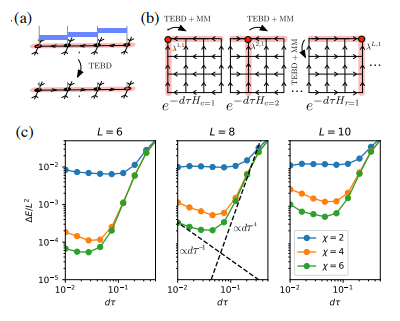
The author also implemented the algorithm. The main idea of TEBD is to use the annealing algorithm based on Trotter-Suzuki decomposition to evolve the randomly initialized MPS state to the ground state, convert the evolution process into a tensor network shrinkage problem, and use the TEBD algorithm to solve the shrinkage . Specifically, a Trotterized time stepper is proposed for isoTNS, which can obtain the ground state through virtual time evolution. Assuming that there is only nearest neighbor interaction, we split the Hamiltonian into terms acting on columns and rows , and then perform Trotterized , as shown in Figure (a). For 1D TEBD updates, it can be easily improved to second order. We start from the orthogonal center, and then gradually move the orthogonal center by calling the standard 1D TEBD algorithm and MM algorithm. In one scan, the algorithm is actually two nested versions of 1D TEBD, hence the name . Among them, the evolution of is achieved by calling 1D TEBD, and its complexity is that of MM , while the complete update complexity of unconstrained PEPS is . Figure (c) shows the energy error density of the g=3.5 transverse field Ising model as a function of Trotter step size for different system sizes and maximum bond dimensions . As the bond size increases, the minimum energy converges toward the exact result.

Efficient quantum state tomography

1. Abstract

Inferring quantum states from measured data becomes infeasible for larger systems because the number of measurements and the amount of computation required to process them grows exponentially with system size. In this article a tomography scheme is proposed that is more advantageous than direct tomography of system size. This method requires uniform manipulation of a constant number of subsystems and relies only on a linear number of experimental manipulations. This scheme can be applied to a wide range of quantum states, especially MPS.

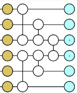
2. Scheme based on unitary transformation

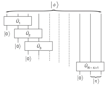
The core idea of this method is to find a sequence of operations to disentangle a chain from left to right. Each operation in this sequence is local and independent of the dimension N.

Assume that the ideal state is , and we assume that this quantum state is an MPS with a given bond dimension of R. The goal of this method is to reconstruct this .

Algorithm process:

(Image source: Nature Communications 1, 149 (2010))

1) First, we take 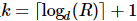, and then do standard quantum state tomography on the first k sites, then the reduced density matrix of the first k sites is: , this reduced density matrix has eigendecomposition , where, . Therefore, there exists a density matrix with one less qudit whose rank R and eigenvalue sum are the same.

2). Then, we further use the information to construct a unitary matrix for the first k positions , which can disentangle the first site.

3). Apply the action to the original state to get: 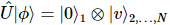Among them, there are some pure states in position.

4). Then repeat the above process for the next 2nd to k+1 positions. By analogy, we can get a sequence of unitary matrices 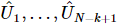, each of which acts at 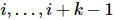positions. This sequence becomes , where each acts in positions. This sequence makes , where , are some pure states at the last k-1 positions.

In summary, this scheme deduces a quantum circuit for preparing MPS. The MPS decomposition can be easily obtained by and .

3. Error
The error of this method mainly comes from two aspects. One is the inability to fully express the quantum state due to the limitation of bond dimension, and the other is the error caused by measurement.

Given an estimated disentangled unitary matrix , an arbitrary state can be expressed as: 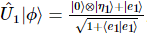, where is the error vector.

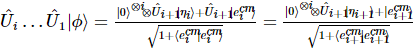
In the next steps, we can get the state in the following form: 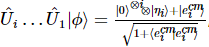, where,

is the cumulative error.

We can truncate this error vector by measuring the first i particles in the standard basis and post-selecting on the result of all zeros. The probability of this happening is roughly , and leaves the system in state .

After a series of unitary transformations, the final state is:

Among them, 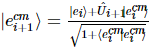, therefore, .

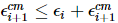We can find that the error accumulates linearly with the number of particles, and the MPS we obtain is recorded as: , then we have:

in, . The overall error is at most the sum of the individual errors at each step.

Essay Lecture | Quantum Computing Two-Dimensional Isometric Tensor Network State

Guess you like