
convolutional neural network
Each convolution kernel extracts different features . Each convolution kernel convolves the input to generate a feature map. This feature map reflects the features extracted by the convolution kernel from the input. Different feature maps show different features in the image.
- Shallow convolution kernel extraction: underlying pixel features such as edges, colors, and patches;
- Middle-level convolution kernel extraction: middle-level texture features such as stripes, lines, shapes, etc.;
- High-level convolution kernel extraction: high-level semantic features such as eyes, tires, text, etc.
Finally, the classification output layer outputs the most abstract classification result.
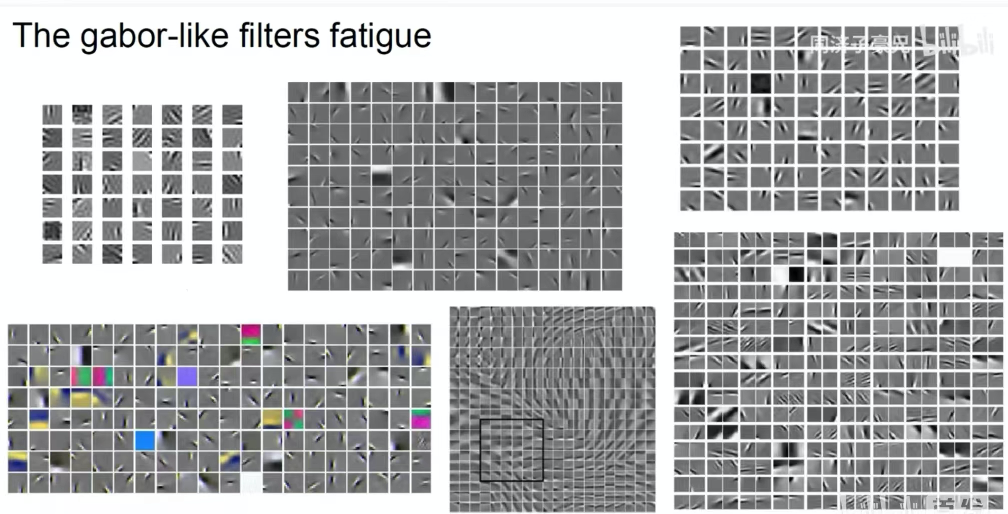
The picture above shows the features extracted by a shallow convolution kernel. We can see that some convolution kernels extract shapes and some extract colors. It is a convolution feature similar to the Gabor filter.
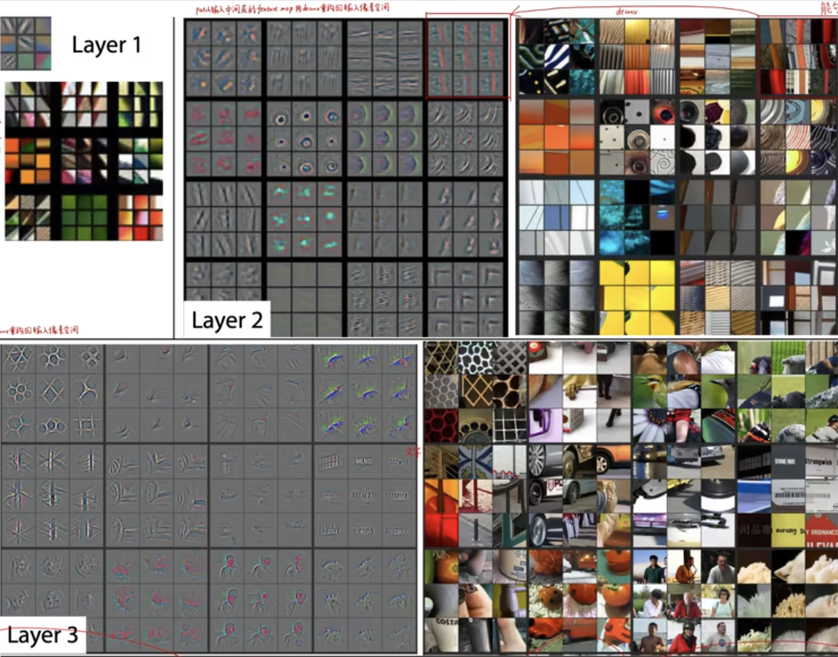
The picture above shows the features extracted by the middle and deep convolution kernels. The middle convolution kernel extracts larger blocks of color and texture; the features extracted by the deep convolution kernel may include humans or some concrete things.
CAM interpretability
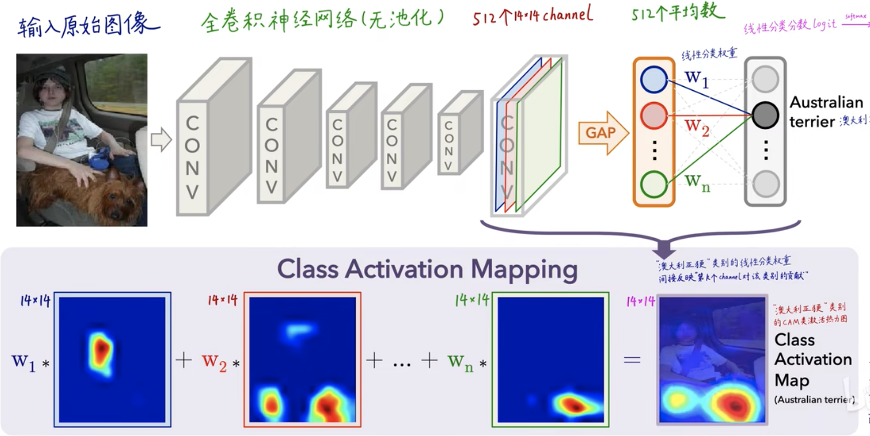
In the figure above, the input original image has been convolved layer by layer. At the last layer, there will be 512 convolution kernels and 512 channels, that is, 512 deep features have been extracted . After GAP (global average pooling), the An average is calculated for each channel feature, and then the weight (coefficient) of each feature value is obtained through the FC (fully connected layer) layer - \(W_1, W_2, W_3,..., W_n\) , for each category You can get a score value (score), which is obtained by
\(score=W_1*blue eigenvalue+W_2*red eigenvalue+...+W_n*green eigenvalue\)
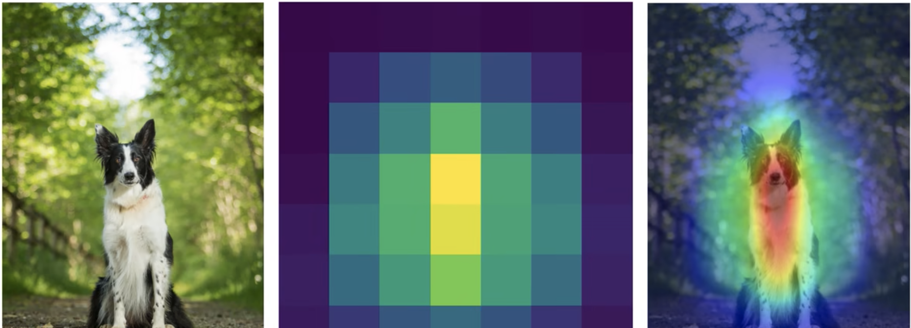
Obtained, and finally calculate a probability value through softmax, which is a process of CNN classification. For CAM heat map, it is mainly reflected in the feature value weight \(W_1, W_2, W_3,..., W_n\) , which indicates the degree of attention that the final classification result pays to different features .
- Disadvantages of CAM
- There must be a GAP layer, otherwise the model structure must be modified and retrained.
- Only the output of the last convolutional layer can be analyzed, and the middle layer cannot be analyzed.
- Image classification tasks only
GradCAM

In GradCAM, instead of using the GAP layer, you can completely use the FC layer to output the score through the fully connected layer, represented by \(y^c\) .
- Derivative of a matrix
1. The derivative of a scalar function with respect to a vector:
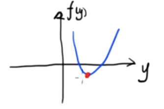
This is a two-dimensional scalar function. We know that the minimum value of this function is
\({df(y)\over dy}=0\)
If this function is a three-dimensional scalar function composed of two independent variables, the image is as follows
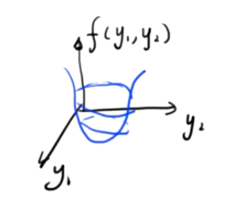
Find the minimum value of this binary function, simultaneously
- \({∂f(y_1,y_2)\over ∂y_1}=0\)
- \({∂f(y_1,y_2)\over ∂y_2}=0\)
If a scalar function has n independent variables \(f(y_1,y_2,y_3,...,y_n)\) , we define a vector
Y=[ ![]() ]
]
Then the partial derivative of the function with respect to the vector Y can be defined as
\({∂f(Y)\over ∂Y}=\)\([\)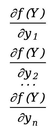 \(]\)
\(]\)
This is an n*1 column vector, and we find that its number of rows is the same as the denominator Y. This layout is called a denominator layout .
Similarly, we can also define the partial derivative of the function with respect to the vector Y as
\({∂f(Y)\over ∂Y}=[{∂f(Y)\over ∂y_1}{∂f(Y)\over ∂y_2}...{∂f(Y)\over ∂y_n}]\)
This is a 1*n row vector, and we find that its number of rows is the same as the numerator f(Y) (a 1*1 scalar). Such a layout is called a numerator layout .
The denominator layout and the numerator layout are the transposes of each other .
Example 1: \(f(y_1,y_2)=y_1^2+y_2^2\)
Denominator layout:
Let Y=[ ![]() ]
]
but
\({∂f(Y)\over ∂Y}=\)[![]() ]=[
]=[![]() ]
]
Molecular layout:
令\(Y=[y_1 y_2]\)
but
\({∂f(Y)\over ∂Y}=[{∂f(Y)\over ∂y_1} {∂f(Y)\over ∂y_2}]=[2y_1 2y_2]\)
2. Derivative of vector function with respect to vector
If our function is also a vector
F(Y)=[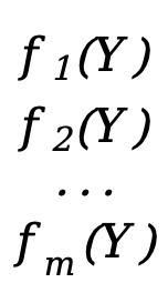 ]
]
Each \(f_x(Y)\) (x=1,2,3,...,m) here is equivalent to a scalar function f(Y) above (the independent variable is the vector Y), F(Y ) is a vector function of m*1.
Example one:
- Y=[
 ]
] - F(Y)=[
 ]=[
]=[ ]
]
The partial derivative of a vector function with respect to a vector, the denominator layout is
\({∂F(Y)\over ∂Y}=\)[ ]=[
]=[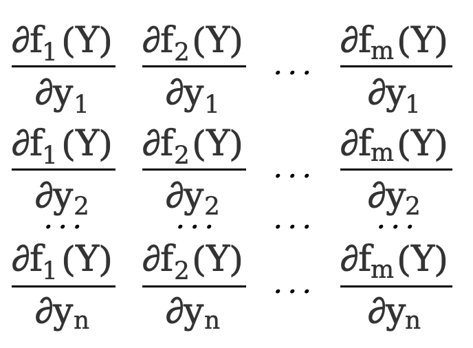 ]
]
As in Example 1, there are
\({∂F(Y)\over ∂Y}=\)[![]() ]=[
]=[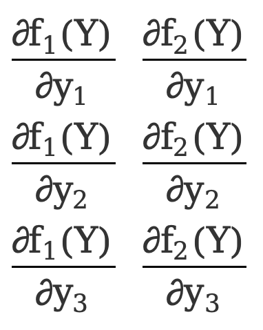 ]=[
]=[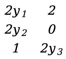 ]
]
This is a 3*2 matrix.
A programmer born in the 1990s developed a video porting software and made over 7 million in less than a year. The ending was very punishing! Google confirmed layoffs, involving the "35-year-old curse" of Chinese coders in the Flutter, Dart and Python teams . Daily | Microsoft is running against Chrome; a lucky toy for impotent middle-aged people; the mysterious AI capability is too strong and is suspected of GPT-4.5; Tongyi Qianwen open source 8 models Arc Browser for Windows 1.0 in 3 months officially GA Windows 10 market share reaches 70%, Windows 11 GitHub continues to decline. GitHub releases AI native development tool GitHub Copilot Workspace JAVA is the only strong type query that can handle OLTP+OLAP. This is the best ORM. We meet each other too late.