Non-intrusive way to build network topology for Kubernetes applications

The open source China community team made its first live broadcast, telling the story behind the open source China community in the name of sharing."

The magic of eBPF code, propagating peer addresses directly into the TCP stream to reconstruct the communication topology

译自Building a network topology of a Kubernetes application in a non-intrusive way，作者 Ilya Shakhat。

introduce

A Kubernetes application is logically divided into two parts: one part is the computing resources (represented by pods), and the other part provides access to the application (represented by services). Application clients can access it using the abstract name without caring about which pod actually handles the request. And, since a single service may have multiple pods as backends, it also acts as a load balancer. In a default Kubernetes deployment, this load balancing function is implemented using very simple iptables or Linux IPVS - both work at the L4 (such as TCP) layer and implement a naive, random-based round-robin mechanism. Of course, cloud providers can also offer more traditional load balancing solutions for exposing applications, but let's start simple.

When we think about the various problems that can occur in applications deployed in Kubernetes, there is a class of problems that require understanding the specific instance of handling client requests. For example: (1) an application Pod is deployed on a host with a poor network connection and takes longer to establish a new connection than other Pods, or (2) a Pod's performance degrades over time , while the performance of other Pods remains stable, or (3) a specific client's request affects application performance. Distributed tracing is often one of the ways to gain insight into issues like this, and obviously it's used to trace the path of a client request to the backend application. Traditionally, distributed tracing requires some form of instrumentation, which may move from manually adding code to fully automated injection into the runtime. But can the same effect be achieved without modifying the client code at all?

To debug the above issue, we basically need two features of distributed tracing: (1) collecting metrics related to request latency, and (2) knowing exactly where each request is going. The first feature can be easily implemented in a non-intrusive way using one of the numerous tools supported by eBPF (a technology that allows dynamically attaching probes to kernel functions), e.g. logging which process established a new connection, Get socket/connection related metrics and even check for retransmissions or malicious connection resets. In the openEuler ecosystem, such a tool is gala-gopher, which provides a large number of different probes, including socket, TCP and L7/HTTP(s) probes. However, the second feature (knowing where an individual request is going) is much more difficult to achieve. In a distributed tracing framework, this is achieved by injecting a span/trace ID into the application payload and then correlating observations from both the client and the backend using the same span ID. Being non-intrusive to the application code means that the same information needs to be injected in a generic way, but doing this to the application protocol is simply not feasible as this would require intercepting the outbound traffic, parsing it, injecting the ID and It's serialized and forwarded. It looks like we just reinvented a service mesh!

Before we continue, let’s take a look at the data available in network monitoring. Here we assume that the monitor will get information from all nodes hosting the application Pod, and then this data will be processed by, for example, Prometheus. Collect them. To achieve this, we need some experimental environment.

test environment

First, we need a deployed multi-node Kubernetes cluster. In Huawei Cloud, the corresponding service is called Cloud Container Engine (CCE).

Then we need a test application, and for this we will use a very simple Python program that accepts an HTTP request and is able to make outgoing HTTP requests to the address specified in the original request. This way we can easily link applications.

These applications will be named with the Latin letters A, B, etc. Application A is deployed as Deployment A and Service A, and so on. The first application will also be exposed to the outside world so that it can be called from the outside.

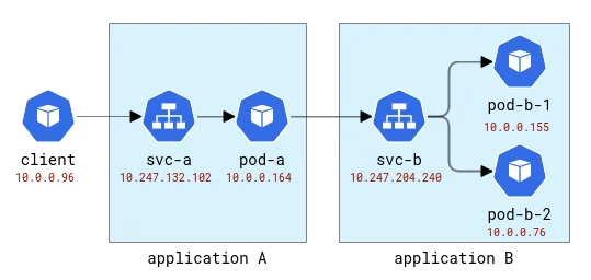
A and B application topology

In Kubernetes Gala-gopher is deployed as a daemon set and runs on every Kubernetes node. It provides metrics that are consumed by Prometheus and ultimately visualized by Grafana. Service topology is built based on metrics and visualized by the NodeGraph plugin.

Observability

Let's send some requests to Application A and forward to Application B like this:

[root@debug-7d8bdd568c-5jrmf /]# curl http://a.app:8000/b.app:8000
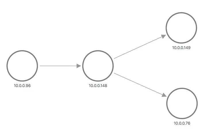
..Hello from pod b-67b75c8557-698tr ip 10.0.0.76 at node 192.168.3.218
Hello from pod a-7954c595f7-tmnx8 ip 10.0.0.148 at node 192.168.3.14

[root@debug-7d8bdd568c-5jrmf /]# curl http://a.app:8000/b.app:8000
..Hello from pod b-67b75c8557-mzn6p ip 10.0.0.149 at node 192.168.3.14
Hello from pod a-7954c595f7-tmnx8 ip 10.0.0.148 at node 192.168.3.14

In the output, we see that one of the requests for Application B was sent to one pod, and the other request was sent to another pod. This is how the topology appears in Grafana:

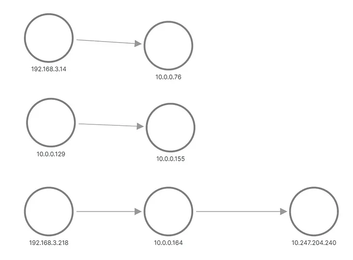
A and B apply topology, reconstructed from metrics

The top and middle rows show something sending a request to Application B's pod, while the bottom shows one of A's pods sending a request to Service B's virtual IP. But this doesn't look like what we expected at all, right? We only see three sets of nodes with no links between them. The IP addresses from the 192.168.3.0/24 subnet are the node addresses from the cluster private network (VPC), and 10.0.0.1/24 is the pod address, except for 10.0.0.129, which is the node address used for intra-node communication .

Now, these metrics are collected at the socket level, which means they are exactly what the application process can see. Collection is done via eBPF probes, so the first idea is to check if the operating system kernel knows more about the application connection than the information available in the socket. The cluster is configured with a default CNI and the Kubernetes service is implemented as an iptables rule. The output of iptables-save shows the configuration. The most interesting ones are these rules that actually configure load balancing:

-A KUBE-SERVICES -d 10.247.204.240/32 -p tcp -m comment 
   --comment "app/b:http-port cluster IP" -m tcp --dport 8000 -j KUBE-SVC-CELO6J2CXNI7KVVA
-A KUBE-SVC-CELO6J2CXNI7KVVA -d 10.247.204.240/32 -p tcp -m comment 
   --comment "app/b:http-port cluster IP" -m tcp --dport 8000 -j KUBE-MARK-MASQ
-A KUBE-SVC-CELO6J2CXNI7KVVA -m comment --comment "app/b:http-port -> 10.0.0.155:8000" 
   -m statistic --mode random --probability 0.50000000000 -j KUBE-SEP-VFBYZLZKPEFJ3QIZ
-A KUBE-SVC-CELO6J2CXNI7KVVA -m comment --comment "app/b:http-port -> 10.0.0.76:8000" 
   -j KUBE-SEP-SXF6FD423VYX6VFB

Load balancing is done on the same node as the client. So if we map pods to nodes it looks like this:

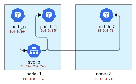
Map A and B application topology to Kubernetes nodes

Internally iptables (actually nftables ) uses the conntrack module to understand that packets belong to the same connection and should be handled in a similar way. Conntrack is also responsible for address translation, so nodes with client applications should know where to send packets. Let's check it out using the conntrack CLI tool.

# node-1
# conntrack -L | grep 8000
tcp      6 82 TIME_WAIT src=10.0.0.164 dst=10.247.204.240 sport=51030 dport=8000 src=10.0.0.76 dst=192.168.3.14 sport=8000 dport=19554 [ASSURED] use=1
tcp      6 79 TIME_WAIT src=10.0.0.164 dst=10.247.204.240 sport=51014 dport=8000 src=10.0.0.155 dst=10.0.0.129 sport=8000 dport=56734 [ASSURED] use=1

# node-2
# conntrack -L | grep 8000
tcp      6 249 CLOSE_WAIT src=10.0.0.76 dst=192.168.3.14 sport=8000 dport=19554 [UNREPLIED] src=192.168.3.14 dst=10.0.0.76 sport=19554 dport=8000 use=1

Okay, so we see that on the first node, the address was translated from Application A's pod and we got a node address with some random port. On the second node, the connection information is reversed as its own packet is actually a reply, but with this in mind we see that the request is coming from the first node and the same random port. Note that there are two requests on Node-1 because we sent 2 requests and they were handled by different pods: pod-b-1 on the same node and pod-b-2 on another node.

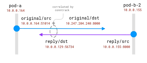
The good news here is that it is possible to know the actual request recipient on the client node, but for the server side it needs to be correlated with the information collected on the client node . like this:

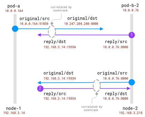
Connections are tracked by the conntrack module. The blue circle is the local address observed in the socket, and the purple one is the remote address. The challenge is to relate purple and blue.

When both client and server pods are on the same node, correlation becomes simpler, but there are still some assumptions about which addresses are real and which should be ignored:

A connection between two Pods on the same node. The source address is real, but the destination address needs to be mapped

Here, the operating system has full visibility into the NAT and can provide a mapping between the real source and the real destination. It is _possible_ to rebuild the complete stream from 10.0.0.164 to 10.0.0.155.

To conclude this section, it should be possible to extend existing eBPF probes to include information about address translation from the conntrack module. The client can know where the request is going. But the server is not always able to know who the client is, there is no centralized correlation algorithm directly. In contrast, distributed tracing methods provide clients and servers with information about their peers, directly and immediately from communication data. So, here comes FlowTracer!

FlowTracer

The idea is simple - transfer data between peers directly within the connection. This is not the first time that such a feature is needed, for example, the HTTP load balancer will insert the X-Forwarded-For HTTP header to let the backend server know about the client. The limitation here is that we want to stay at L4, thus supporting any application level protocol. Such functionality also exists, and some L4 load balancers (such as this one ) can inject the origin address as a TCP header option and make it available to the server.

Summary of requirements:

L4 layer transport peer address.
Ability to dynamically enable address injection (as easily deploying applications in K8s).
Non-invasive and fast.

The most straightforward approach seems to be to use TCP header options (also known as TOA). The payload is the IP address and port number (because they change during address translation). Since Huawei Kubernetes deployment only supports IPv4, we can limit support to only IPv4. IPv4 addresses are 32 bits, while port numbers require 16 bits, requiring a total of 6 bytes, plus 1 byte for the option type and 1 byte for the option length. Here is what the TCP header specs look like:

The header can contain multiple options up to 40 bytes. Each option can have variable length and type/kind.

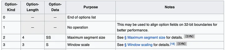
In general, Linux TCP packets already have some options, such as MSS or timestamp. But there are still about 20 bytes of space available for us.

Now, when we know where to put the data, the next question is where should we add the code? We want the solution to be as general as possible and can be used for all TCP connections. The ideal place is somewhere in the kernel in the network stack, in what's called a socket buffer (a structure that represents network connection information), from the top level all the way down to packets ready to be transmitted over the network. From an implementation perspective, the code should be eBPF code (of course!) and address injection functionality can then be enabled dynamically.

The most obvious place for this kind of code is TC, a flow control module. At the TC, the eBPF program has access to the created packet, and it can read and write data from the packet. One disadvantage is that the packet needs to be parsed from the beginning, that is, even though the bpf_skb_load_bytes_relative function provides a pointer to the beginning of the L3 header, the L4 position still needs to be calculated manually. The most problematic is the insert operation. There are 2 functions with promising names, bpf_skb_adjust_room and bpf_skb_change_tail , but they allow up to L3 packet resizing, not L4. An alternative solution is to check if the existing TCP header contains certain options and override them, but let's first check what a typical packet contains.

1514772378.301862 IP (tos 0x0, ttl 64, id 20960, offset 0, flags [DF], proto TCP (6), length 60)
    192.168.3.14.28301 > 10.0.0.76.8000: Flags [S], cksum 0xbc03 (correct), seq 1849406961, win 64240, options [mss 1460,sackOK,TS val 142477455 ecr 0,nop,wscale 9], length 0
        0x0000:  0000 0001 0006 fa16 3e22 3096 0000 0800  ........>"0.....
        0x0010:  4500 003c 51e0 4000 4006 1ada c0a8 030e  E..<Q.@.@.......
        0x0020:  0a00 004c 6e8d 1f40 6e3b b5f1 0000 0000  ...Ln..@n;......
        0x0030:  a002 faf0 bc03 0000 0204 05b4 0402 080a  ................
        0x0040:  087e 088f 0000 0000 0103 0309            .~..........

This is the TCP SYN packet sent when the client establishes a connection with the backend application. The header contains several options: MSS to specify the maximum segment size, then optional acknowledgment, a specific timestamp to ensure the order of packets, an opcode NOP possibly for word alignment, and finally for alignment Window scaling for window size. From that list, the timestamp option is the best candidate to be covered (according to Wikipedia, adoption is still around 40%), while DeepFlow - one of the leaders in non-intrusive eBPF tracking - has This operation was performed in .

While this approach seems feasible, it is not easy to implement. The TC program has access to translated addresses, which means that the translation map should somehow be retrieved from the conntrack module and stored. The TC program attaches to the network card, so if a node has multiple network cards, the deployment needs to correctly identify the attachment location. The reader module has to parse all the packets to find the TCP and then iterate through the headers to find where our header is. Is there any other way?

When searching for this question via Google in August 2023, it’s common to see No More Results at the bottom of the search results page (hopefully this blog post will change that!). The most useful reference is a link to a Linux Kernel patch produced by Facebook engineers in 2020. This patch shows what we're looking for:

Early work on BPF-TCP-CC allowed TCP congestion control algorithms to be written in BPF. It provides the opportunity to improve turnaround time in production environments when testing/releasing new congestion control ideas. The same flexibility can be extended to writing TCP header options.

It's not unusual for people to want to test new TCP header options to improve TCP performance. Another use case is for data centers that have a more controlled environment and can put header options in internal-only traffic, which gives more flexibility.

The holy grail are these functions: bpf_store_hdr_opt and bpf_load_hdr_opt ! Both belong to a special type of sock ops program, available since the 5.10 kernel, meaning that they can be used in almost any version after 2022. The Sock ops program is a single function attached to cgroup v2 that allows it to be enabled only for certain sockets (for example, belonging to a specific container). The program receives a single operation indicating the current state of the socket. When we want to write a new header option, we first need to enable writing for an active or passive connection, and then we need to tell the new header length before the header payload can be written. The read operation is simpler, however, we also need to enable reading first before we can read the header options. When a TCP packet is created, the TCP header callback is called. This happens before address translation, so we can copy the socket source address into the header options. The reader can easily extract the value from the header option and store it in a BPF map so that later, the consumer can read and map from the observed remote address to the actual address. The BPF portion of the first run code is far less than 100 lines. Pretty good!

Make code production-ready

However, the devil is in the details. First, we need a way to delete old records from the BPF map. The best time to do this is when the conntrack module deletes the connection from its table. This article by Arthur Chiao provides a good description of the conntrack module and the internal structure of the connection lifecycle, so it is easy to find the correct function in the kernel sources - nf_conntrack_destroy . This function receives the conntrack entry before deleting it from the internal table. Since this is when the connection officially ends, we can also add a probe that will also remove the connection from our mapping table.

In the sock ops program, we do not specify into which packets the new header option is injected, assuming it applies to all packets. In fact, this is true, but the read is only effective when the connection is in the established/acknowledged state, which means that the server side cannot read the header options from the incoming SYN packet. SYN-ACK is also processed before the regular TCP stack, and header options can neither be injected nor read. In fact, this feature only works on both ends if the connection runs entirely with the first PSH (packet). This is perfectly fine for a working connection, but if the connection attempt fails, the client doesn't know where it was trying to connect to. This is a critical mistake; this information is useful for debugging network problems. As we know, Kubernetes load balancing is implemented on the client node, so we can extract the information from conntrack and store it in the same format as the data received through the stream. The Conntrack function ___nf_conntrack_confirm_ helps here - it is called when a new connection is about to be confirmed, which for active client (outgoing) TCP connections occurs when the first SYN packet is sent.

With all these additions, the code becomes a bit bloated, but still far less than 1000 lines in total. The full patch is available in this MR . Time to enable it in our experiment setup and check the metrics and topology again!

Look:

Correct A/B application topology

This article was first published on Yunyunzhongsheng ( https://yylives.cc/ ), everyone is welcome to visit.