Introduction : ArcGraph is a distributed graph database with cloud-native architecture and integrated storage, query and analysis. This article will explain in detail how ArcGraph can flexibly handle graph analysis under limited memory.

01 Introduction

As graph analysis technology is widely used, academia and major graph database vendors are keen to improve the high performance indicators of graph analysis technology. However, in the pursuit of high-performance computing, the method of "trading space for time" is often adopted, that is, accelerating computing by increasing memory usage. However, at this stage, external memory graph computing is not yet mature, and graph analysis still relies on full memory computing, which leads to a strong dependence of high-performance graph computing engines on large memory. When there is insufficient memory, graph analysis tasks cannot be executed.

We have found from many past customer cases that the hardware resources invested by customers in graph analysis are usually fixed and limited, and the resources of the test environment are more limited than those of the production environment. Customers usually require the timeliness of graph analysis to be T+1, which is a typical offline analysis requirement. Therefore, customers expect graph computing engines to reduce the demand for resources such as CPU and memory, and not pursue high algorithm performance too much, as long as T+1 is met. This is a big challenge for most graph computing engines. The demand for CPU is relatively easy to control, while the demand for memory is difficult to significantly optimize in a short R&D cycle.

ArcGraph also faces the above challenges, but through continuous summarization and polishing in customer delivery practices, its graph computing engine has the flexibility to balance processing in time and space. At present, ArcGraph's built-in graph computing engine is in the leading position in the industry in terms of graph analysis performance indicators, and is still being optimized and improved. Next, we will explain how ArcGraph cleverly uses time to exchange space to deal with graph analysis under limited memory from multiple angles, such as the underlying data structure of the engine and the call of the upper-level algorithm.

02 Select the type of point ID

ArcGraph 图计算引擎支持三种点 ID 类型：string、int64、int32。string点类型的支持，可提高对源数据的兼容性，但相对于 int64 而言，因为需要在内存中维护一份 string 到 int64 的点 id 映射表，会增加内存使用量。若指定点类型为 int64，则 ArcGraph 会将源数据中的 string 类型点 ID 生成一份 int64 映射表，并置于外存中，内存中只保留映射后的int64 类型点边数据。待计算完成后，再将映射表读入内存做 string id 还原。因此，使用 int64 类型的点 ID，会增加用于映射表在外存与内存间交换的额外时间消耗，但也会显著降低整体的内存使用量，节省的内存大小取决于原始 ID 的长度及点数据量。

In addition, the ArcGraph graph computing engine also supports int32. For scenarios where the total number of source data points is less than 40 million, it can further reduce memory usage by about 30% compared to int64.

The following is an example of specifying the type of the point ID in the ArcGraph Execute Graph Algorithm API:

curl -X 'POST'   'http://myhost:18000/graph-computing?reload=true&use_cache=true'   -H 'accept: application/json'   -H 'Content-Type: application/json'   -d '{
    "algorithmName": "pagerank",
    "graphName": "twitter2010",
    "taskId": "pagerank",
    "oid_type": "int64", 
    "subGraph": {
      "edgeTypes": [
        {
          "edgeTypeName": "knows",
          "props": [],
          "vertexPairs": [
            {
              "fromName": "person",
              "toName": "person"
            }
          ]
        }
      ],
      "vertexTypes": [
        {
          "vertexTypeName": "person",
          "props": []
        }
      ]
    },
    "algorithmParams": {
    }
  }'

03 Enable Varint encoding

Varint encoding is used to compress and encode integers. It is a variable-length encoding method. Taking int32 as an example, it takes 4 bytes to store a value normally. In conventional Varint encoding, the last 7 bits of each byte represent data, and the highest bit is the flag bit.

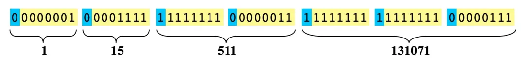
If the highest bit is 0, it means that the last 7 bits of the current byte are all the data, and the subsequent bytes are irrelevant to the data. For example, the integer 1 in the figure above only needs one byte to represent: 00000001, and the subsequent bytes do not belong to the data of the integer 1.
If the highest bit is 1, it means that the subsequent bytes are still part of the data. For example, the integer 511 in the figure above requires 2 bytes to represent: 11111111 00000011, and the subsequent bytes are the data of 131071.

Using this idea, 32-bit integers can be represented by 1-5 bytes. Correspondingly, 64-bit integers can be represented by 1-10 bytes. In actual usage scenarios, the usage rate of small numbers is much higher than that of large numbers, especially for 64-bit integers. Therefore, Varint encoding can usually achieve a significant compression effect. There are multiple variants of Varint encoding, and there are also many open source implementations.

ArcGraph 图计算引擎支持使用 Varint 编码来压缩内存中的边数据存储（主要为 CSR/CSC）。当开启 Varint 编码后，边数据所占内存可显著降低，实测可达 50%左右。同时，因编解码带来的性能损耗也会高达 20%左右。因此，在开启前，需要清晰了解使用场景和客户需求，确保因节省内存而带来的性能损耗在可接受范围内。

The following is an example of Varint encoding to enable graph computation in ArcGraph's graph loading API:

curl -X 'POST'   'http://localhost:18000/graph-computing/datasets/twitter2010/load'   -H 'accept: application/json'   -H 'Content-Type: application/json'   -d '{
    "oid_type": "int64",
    "delimeter": ",",
    "with_header": "true",
    "compact_edge": "true"
  }'

04 Enable Perfect HashMap

The difference between Perfect HashMap and other HashMaps is that it uses Perfect Hash Function (PHF). Function H maps N key values to M integers, where M>=N, and satisfies H(key1)≠H(key2)∀key1,key2, then the function is a perfect hash function. If M=N, then H is the Minimal Perfect Hash Function (MPHF). At this time, N key values will be mapped to N consecutive integers.

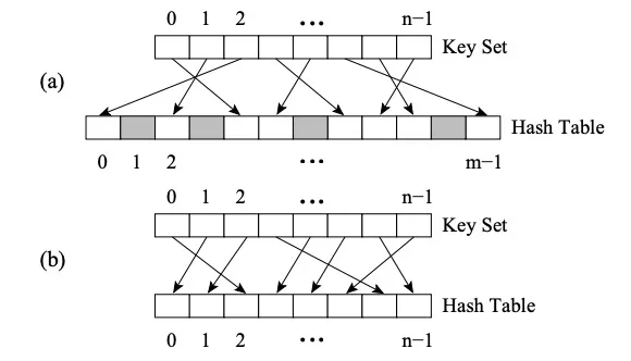Figure (a) is PHF, Figure (b) is MPHF

The figure above is the FKS strategy of two-level hashing. First, the data is mapped to the T space through the first-level hashing, and then the conflicting data is randomly mapped to the S space using a new hash function, and the size of the S space m is the square of the conflicting data (for example, if three numbers in T2 conflict, they are mapped to the S2 space where m is 9). At this time, it is easy to find a hash function that avoids collisions. By appropriately selecting a hash function to reduce collisions during the first-level hashing, the expected storage space can be O (n).

The ArcGraph graph computing engine maintains a mapping from the original point ID to the internal point ID in memory. The internal points are continuous long integer types, which facilitates data compression and vectorization optimization. The mapping is essentially a hashmap, but ArcGraph provides two methods for the underlying implementation:

Flat HashMap - The advantage is that it is fast to build, but the disadvantage is that it usually requires more memory space to reduce frequent hash collisions.
Perfect HashMap - The advantage is that less memory is used to ensure worst-case O(1) efficiency queries, but the disadvantage is that all keys need to be known in advance and the construction time is long.

Therefore, turning on Perfect HashMap can also achieve the goal of trading time for space. According to the test, for the mapping set from original points to internal point IDs, the memory usage of Perfect HashMap is usually only about 1/5 of that of Flat HashMap, but correspondingly, its construction time is also 2-3 times that of Flat HashMap.

The following is an example of a Perfect HashMap that enables graph computation in ArcGraph's graph loading API:

curl -X 'POST'   'http://localhost:18000/graph-computing/datasets/twitter2010/load'   -H 'accept: application/json'   -H 'Content-Type: application/json'   -d '{
    "oid_type": "int64",
    "delimeter": ",",
    "with_header": "true",
    "compact_edge": "true",
    "use_perfect_hash": "true"
  }'

05 Optimization algorithm implementation and result processing

The memory usage at the algorithm implementation level depends on the specific logic of the algorithm. We have summarized the following points from practice to achieve the goal of trading time for space:

Appropriately reduce the use of multi-threaded processing and ThreadLocal objects in the algorithm. The algorithm often involves the storage of temporary vertex-edge sets. If these storages appear in multi-threaded logic, the overall memory will increase with the number of threads. Appropriately reducing the number of concurrent threads or reducing the use of ThreadLocal large objects will help reduce memory. Appropriately increase the data exchange between internal and external memory. According to the specific logic of the algorithm, serialize the temporarily unused large objects into the external memory, and when using the object, read it into the memory in a streaming manner to avoid multiple large objects occupying a large amount of memory at the same time.

The following is an example of an algorithm implementation that reflects the above two points:

void IncEval(const fragment_t& frag, context_t& ctx,
               message_manager_t& messages) {
    ...
    ...    
    if (ctx.stage == "Compute_Path"){  
        auto vertex_group = divide_vertex_by_type(frag);

        //此处采用单线程for循环而非多线程并行处理，意在防止多个path_vector同时占内存导致OOM。
        for(int i=0; i < vertex_group.size(); i++){

            //此处path_vector是每个group中任意两点间的全路径，可理解为一个超大对象
            auto path_vector = compute_all_paths(vertex_group[i]);

            //拿到该对象后不会在当前stage使用，所以先序列化到外存中。
            serialize_path_vector(path_vector, SERIALIZE_FOLDER);
        }
        ...
        ...
    }
    ...
    ...
    if (ctx.stage == "Result_Collection"){

        //在当前stage中，将之前stage生成的多个序列化文件合并为一个文件，并把文件路径返回。
        auto result_file_path = merge_path_files(SERIALIZE_FOLDER);
        ctx.set_result(result_file_path);
        ...
        ...
    }
    ...
    ...
 }

After the calculation is completed, the results are written to the external memory and the related memory of the graph computing engine is released. In some scenarios, the result processing program will run on the graph computing cluster server to read the graph computing results and further process them. If the graph computing engine memory has not released the calculation results, in the worst case, there will be two copies of the result data in the current server memory. In the case of large data volume, one copy of the result data will occupy a very high memory. Therefore, in such scenarios, it is necessary to give priority to writing the calculation results to the external memory and releasing the graph computing engine memory in time.

At the same time, the ArcGraph team will continue to challenge the "both" of high performance and low resource usage, and work with academic and industry partners to further refine the image memory and computing efficiency to achieve further technological breakthroughs.

Using time to trade space: How ArcGraph can flexibly cope with graph analysis under limited memory

01 Introduction

02 Select the type of point ID

03 Enable Varint encoding

04 Enable Perfect HashMap

05 Optimization algorithm implementation and result processing

Guess you like