Depth study into the pit of the four notes --- Film Critics text classification

Disclaimer: This article is a blogger original article, follow the CC 4.0 BY-SA copyright agreement, reproduced, please attach the original source link and this statement.

This link: https://blog.csdn.net/LEEANG121/article/details/102491037

Movie critics are generally divided into positive (positive) or negative (nagetive) categories. This is a binary (binary) or binary classification, an important and widely used machine learning problems.
We will use the IMDB data set (IMDB dataset) comes from the Internet Movie Database (Internet Movie Database), which contains 50,000 pieces critic text. Cut out from the data set used for training reviews 25,000, 25,000 as additional testing. Training set and test set are balanced (balanced), meaning that they contain an equal number of positive and negative comments.
Tensorflow code for this article from the official website tutorial

Download Data

And before the project, first configure the environment parameters specific code is as follows:

from __future__ import absolute_import, division, print_function, unicode_literals#该行要放在第一行位置
import warnings#忽略系统警告提示
warnings.filterwarnings('ignore')
import tensorflow as tf
from tensorflow import keras

import numpy as np
print(tf.__version__)

2.0.0

After the basic configuration is set up and download the data set. IMDB data set has been packed in the Tensorflow. The data set has been subjected to pretreatment, Comments (word sequence) that has been converted into a sequence of integers where each integer represents a particular word in the dictionary. Specific code as follows:

imdb = keras.datasets.imdb
(train_data, train_labels), (test_data, test_labels) = imdb.load_data(num_words=10000)#参数 num_words=10000 保留了训练数据中最常出现的 10,000 个单词。为了保持数据规模的可管理性，低频词将被丢弃。

Parameters num_words = 10000 retained the 10,000 words in the training data most frequently occurring, note 10 000 refers to the number of samples the number of common words, not a download. In order to maintain manageable data size, low-frequency words will be discarded.
Here if you have already downloaded the data sets are copied directly from the cache.

Understanding Data
Let's take a moment to understand the data format. The data set is pre-processed: each sample is an array of integers critic Vocabulary FIG. Each tag is an integer value of 0 or 1, where 0 represents negative comments, represents a positive comments.

print('Training entries: {}, labels: {}'.format(len(train_data), len(train_labels)))

Training entries: 25000, labels: 25000#25000个样本和25000个标签

Review text is converted to an integer value, wherein each integer represents a word dictionary. ( Note: here I would have thought that each number represents 26 letters in a ... this is the literal meaning of a word, I will describe specific detail below ) Our first comment as an example:

print(train_data[0]) #这里一定要注意，每个数字代表的是单词，不是字母。

[1, 14, 22, 16, 43, 530, 973, 1622, 1385, 65, 458, 4468, 66, 3941, 4, 173, 36, 256, 5, 25, 100, 43, 838, 112, 50, 670, 2, 9, 35, 480, 284, 5, 150, 4, 172, 112, 167, 2, 336, 385, 39, 4, 172, 4536, 1111, 17, 546, 38, 13, 447, 4, 192, 50, 16, 6, 147, 2025, 19, 14, 22, 4, 1920, 4613, 469, 4, 22, 71, 87, 12, 16, 43, 530, 38, 76, 15, 13, 1247, 4, 22, 17, 515, 17, 12, 16, 626, 18, 2, 5, 62, 386, 12, 8, 316, 8, 106, 5, 4, 2223, 5244, 16, 480, 66, 3785, 33, 4, 130, 12, 16, 38, 619, 5, 25, 124, 51, 36, 135, 48, 25, 1415, 33, 6, 22, 12, 215, 28, 77, 52, 5, 14, 407, 16, 82, 2, 8, 4, 107, 117, 5952, 15, 256, 4, 2, 7, 3766, 5, 723, 36, 71, 43, 530, 476, 26, 400, 317, 46, 7, 4, 2, 1029, 13, 104, 88, 4, 381, 15, 297, 98, 32, 2071, 56, 26, 141, 6, 194, 7486, 18, 4, 226, 22, 21, 134, 476, 26, 480, 5, 144, 30, 5535, 18, 51, 36, 28, 224, 92, 25, 104, 4, 226, 65, 16, 38, 1334, 88, 12, 16, 283, 5, 16, 4472, 113, 103, 32, 15, 16, 5345, 19, 178, 32]

Movie reviews may have different lengths. The following code shows the number of words in the first and second reviews. Since the input of the neural network must be uniform length, we need to solve this problem later.

len(train_data[0]), len(train_data[1])

(218, 189)

The integer word is converted back
to a string of numbers represents the specific meaning of the above, it must be very curious. Learn how to integer conversion back to the text that you might be helpful. Here we will create a helper function to query a dictionary object that contains the mapping of integer to a string:

#一个映射单词到整数索引的词典
word_index = imdb.get_word_index()#建立词典索引
#保留第一个索引
word_index = {k:(v+3) for k,v in word_index.items()}
word_index["<PAD>"] = 0#这里0代表<PAD>
word_index["<START>"] = 1#这里1代表<START>
word_index["<UNK>"] = 2#这里2代表<UNK>（unknown)
word_index["<UNUSED>"] = 3#这里3代表<UNUSED>

reverse_word_index = dict([(value, key) for (key, value) in word_index.items()])
def decode_review(text):
    return ' '.join([reverse_word_index.get(i, '?') for i in text])

After the establishment of the dictionary is finished, we can use the function to display text decode_review's first comment:

decode_review(train_data[0])

"<START> this film was just brilliant casting location scenery story direction everyone's really suited the part they played and you could just imagine being there robert <UNK> is an amazing actor and now the same being director <UNK> father came from the same scottish island as myself so i loved the fact there was a real connection with this film the witty remarks throughout the film were great it was just brilliant so much that i bought the film as soon as it was released for <UNK> and would recommend it to everyone to watch and the fly fishing was amazing really cried at the end it was so sad and you know what they say if you cry at a film it must have been good and this definitely was also <UNK> to the two little boy's that played the <UNK> of norman and paul they were just brilliant children are often left out of the <UNK> list i think because the stars that play them all grown up are such a big profile for the whole film but these children are amazing and should be praised for what they have done don't you think the whole story was so lovely because it was true and was someone's life after all that was shared with us all"

data processing

Prepare data
due to the input of neural network must be a tensor form, so critics need to first convert tensor, before you can learn, the conversion of two ways:
1 array is converted to indicate the presence or absence of the word 0 and 1 vector composition, similar to one-hot encoding. For example, the sequence [3, 5] is converted to a vector of dimension 10,000, in addition to an index of the vector 3 and 5 is other than 1, the other is 0. Then, as the first floor in a network - a dense layer can handle floating-point vector data. However, this method requires a lot of memory, you need a size num_words * num_reviews matrix.
2 we can fill the array to ensure that the input data having the same length, size and create a integer of max_length * num_reviews tensor. We can use this embedded layer shape data can be processed as a first layer in the network.

In this example, we will use the second method.
As the movie reviews length must be the same, we will use pad_sequences function to standardize the length:

#训练数据长度设置为256
train_data = keras.preprocessing.sequence.pad_sequences(train_data,
                                                        value=word_index["<PAD>"],
                                                        padding='post',
                                                         maxlen=256)
#测试数据长度设置为256
test_data = keras.preprocessing.sequence.pad_sequences(test_data,
                                                       value=word_index["<PAD>"],
                                                       padding='post',
                                                        maxlen=256)

Now let's look at a sample length:

len(train_data[0]), len(train_data[1])

(256, 256)

Let us examine the first comments (currently already filled)

print(train_data[0])

[   1   14   22   16   43  530  973 1622 1385   65  458 4468   66 3941
4  173   36  256    5   25  100   43  838  112   50  670    2    9
35  480  284    5  150    4  172  112  167    2  336  385   39    4
172 4536 1111   17  546   38   13  447    4  192   50   16    6  147
2025   19   14   22    4 1920 4613  469    4   22   71   87   12   16
43  530   38   76   15   13 1247    4   22   17  515   17   12   16
626   18    2    5   62  386   12    8  316    8  106    5    4 2223
5244   16  480   66 3785   33    4  130   12   16   38  619    5   25
124   51   36  135   48   25 1415   33    6   22   12  215   28   77
52    5   14  407   16   82    2    8    4  107  117 5952   15  256
4    2    7 3766    5  723   36   71   43  530  476   26  400  317
46    7    4    2 1029   13  104   88    4  381   15  297   98   32
2071   56   26  141    6  194 7486   18    4  226   22   21  134  476
26  480    5  144   30 5535   18   51   36   28  224   92   25  104
4  226   65   16   38 1334   88   12   16  283    5   16 4472  113
103   32   15   16 5345   19  178   32    0    0    0    0    0    0
0    0    0    0    0    0    0    0    0    0    0    0    0    0
0    0    0    0    0    0    0    0    0    0    0    0    0    0
0    0    0    0]

Now you can see the data length are 256.

Model building

Network architecture model
next model were built, the neural network is constructed of stacked layers, which need to architectural decisions from two main aspects:
model, there are many layers?
Each layer in the number of hidden units (hidden units)?
In this sample, the input data comprising an array of word indices. Label to be predicted is 0 or 1. Let's build a model for this problem, we first use keras.Sequential be serialized to add layers, the specific code as follows:

# 输入形状是用于电影评论的词汇数目（10,000 词）
vocab_size = 10000
model = keras.sequential()#搭建层
model.add(keras.layers.Embedding(vocab_size, 16))#embedding 是一个将单词向量化的函数，嵌入（embeddings）输出的形状都是：(num_examples, embedding_dimension)
model.add(keras.layers.GloabAveragePooling1D())#添加全局平均池化层
model.add(keras.layers.Dense(16, activation = 'relu'))
model.add(keras.layers.Dense(1, activation = 'sigmoid'))

model.summary()

Model: "sequential"
_________________________________________________________________
Layer (type)                 Output Shape              Param #   
=================================================================
embedding (Embedding)        (None, None, 16)          160000    
_________________________________________________________________
global_average_pooling1d (Gl (None, 16)                0         
_________________________________________________________________
dense (Dense)                (None, 16)                272       
_________________________________________________________________
dense_1 (Dense)              (None, 1)                 17        
=================================================================
Total params: 160,289
Trainable params: 160,289
Non-trainable params: 0

Layer are sequentially stacked to construct classifiers:

The first layer is embedded (Embedding) layer. The layer with integer encoding vocabulary, each word and vector lookup index embedded (embedding vector). These vectors are learned through model training. Vector adds a dimension to the output array. The resulting dimension is: (batch, sequence, embedding) .
embedding the word is a function of the quantization, embedding (embeddings) shape of the output are: (num_examples, embedding_dimension)

Next, GlobalAveragePooling1D will return to a fixed length output vector for each sample by averaging sequence dimensions. This allows the model to the simplest possible way to deal with variable-length input.

The fixed-length output vector through a full transport layer connection (Dense) 16 units of the hidden layer.

Finally, a single layer of output nodes connected dense. Use Sigmoid activation function, a function of the value of floating point numbers between 0 and 1, represents the probability or confidence.
Model Compiler

model.compile(optimize = 'adam',
              loss = 'binary_crossentropy',
              metrics = ['accuracy'])

Model Assessment

Verification Model

x_val = train_data[:10000]#取训练数据集前10000个进行训练和验证
partial_x_train = train_data[10000:]
y_val = train_labels[:10000]#同理取前10000个标签
partial_y_train = train_labels[10000:]

Model training

#以 512 个样本的 mini-batch 大小迭代 40 个 epoch 来训练模型。这是指对 x_train 和 y_train 张量中所有样本的的 40 次迭代。在训练过程中，监测来自验证集的 10,000 个样本上的损失值（loss）和准确率（accuracy）：
history = model.fit(partial_x_train,
                    partial_y_train,
                    epochs=40,
                    batch_size=512,
                    validation_data=(x_val, y_val),
                    verbose=1)

Train on 15000 samples, validate on 10000 samples
Epoch 1/40
15000/15000 [==============================] - 1s 88us/sample - loss: 0.6924 - accuracy: 0.6045 - val_loss: 0.6910 - val_accuracy: 0.6819
Epoch 2/40
15000/15000 [==============================] - 0s 22us/sample - loss: 0.6885 - accuracy: 0.6392 - val_loss: 0.6856 - val_accuracy: 0.7129
Epoch 3/40
15000/15000 [==============================] - 0s 22us/sample - loss: 0.6798 - accuracy: 0.7371 - val_loss: 0.6747 - val_accuracy: 0.7141
Epoch 4/40
15000/15000 [==============================] - 0s 22us/sample - loss: 0.6629 - accuracy: 0.7648 - val_loss: 0.6539 - val_accuracy: 0.7597
Epoch 5/40
15000/15000 [==============================] - 0s 21us/sample - loss: 0.6356 - accuracy: 0.7860 - val_loss: 0.6239 - val_accuracy: 0.7783
Epoch 6/40
15000/15000 [==============================] - 0s 22us/sample - loss: 0.5975 - accuracy: 0.8036 - val_loss: 0.5849 - val_accuracy: 0.7931
Epoch 7/40
15000/15000 [==============================] - 0s 22us/sample - loss: 0.5525 - accuracy: 0.8195 - val_loss: 0.5421 - val_accuracy: 0.8076
Epoch 8/40
15000/15000 [==============================] - 0s 22us/sample - loss: 0.5025 - accuracy: 0.8357 - val_loss: 0.4961 - val_accuracy: 0.8245
Epoch 9/40
15000/15000 [==============================] - 0s 22us/sample - loss: 0.4541 - accuracy: 0.8537 - val_loss: 0.4555 - val_accuracy: 0.8392
Epoch 10/40
15000/15000 [==============================] - 0s 22us/sample - loss: 0.4114 - accuracy: 0.8672 - val_loss: 0.4211 - val_accuracy: 0.8469
Epoch 11/40
15000/15000 [==============================] - 0s 22us/sample - loss: 0.3753 - accuracy: 0.8775 - val_loss: 0.3938 - val_accuracy: 0.8531
Epoch 12/40
15000/15000 [==============================] - 0s 22us/sample - loss: 0.3451 - accuracy: 0.8859 - val_loss: 0.3713 - val_accuracy: 0.8600
Epoch 13/40
15000/15000 [==============================] - 0s 21us/sample - loss: 0.3201 - accuracy: 0.8924 - val_loss: 0.3540 - val_accuracy: 0.8665
Epoch 14/40
15000/15000 [==============================] - 0s 22us/sample - loss: 0.2990 - accuracy: 0.8983 - val_loss: 0.3397 - val_accuracy: 0.8712
Epoch 15/40
15000/15000 [==============================] - 0s 23us/sample - loss: 0.2809 - accuracy: 0.9037 - val_loss: 0.3290 - val_accuracy: 0.8735
Epoch 16/40
15000/15000 [==============================] - 0s 22us/sample - loss: 0.2649 - accuracy: 0.9095 - val_loss: 0.3197 - val_accuracy: 0.8766
Epoch 17/40
15000/15000 [==============================] - 0s 22us/sample - loss: 0.2508 - accuracy: 0.9131 - val_loss: 0.3121 - val_accuracy: 0.8792
Epoch 18/40
15000/15000 [==============================] - 0s 22us/sample - loss: 0.2379 -               accuracy: 0.9183 - val_loss: 0.3063 - val_accuracy: 0.8797
Epoch 19/40
15000/15000 [==============================] - 0s 22us/sample - loss: 0.2262 - accuracy: 0.9216 - val_loss: 0.3013 - val_accuracy: 0.8806
Epoch 20/40
15000/15000 [==============================] - 0s 21us/sample - loss: 0.2156 -   accuracy: 0.9261 - val_loss: 0.2972 - val_accuracy: 0.8828
Epoch 21/40
15000/15000 [==============================] - 0s 22us/sample - loss: 0.2061 - accuracy: 0.9292 - val_loss: 0.2939 - val_accuracy: 0.8827
Epoch 22/40
15000/15000 [==============================] - 0s 22us/sample - loss: 0.1966 - accuracy: 0.9329 - val_loss: 0.2918 - val_accuracy: 0.8833
Epoch 23/40
15000/15000 [==============================] - 0s 21us/sample - loss: 0.1881 - accuracy: 0.9368 - val_loss: 0.2892 - val_accuracy: 0.8837
Epoch 24/40
15000/15000 [==============================] - 0s 22us/sample - loss: 0.1802 - accuracy: 0.9408 - val_loss: 0.2884 - val_accuracy: 0.8841
Epoch 25/40
15000/15000 [==============================] - 0s 21us/sample - loss: 0.1725 - accuracy: 0.9436 - val_loss: 0.2871 - val_accuracy: 0.8845
Epoch 26/40
15000/15000 [==============================] - 0s 22us/sample - loss: 0.1656 - accuracy: 0.9468 - val_loss: 0.2863 - val_accuracy: 0.8856
Epoch 27/40
15000/15000 [==============================] - 0s 22us/sample - loss: 0.1592 - accuracy: 0.9494 - val_loss: 0.2863 - val_accuracy: 0.8862
Epoch 28/40
15000/15000 [==============================] - 0s 21us/sample - loss: 0.1529 - accuracy: 0.9516 - val_loss: 0.2868 - val_accuracy: 0.8851
Epoch 29/40
15000/15000 [==============================] - 0s 21us/sample - loss: 0.1465 - accuracy: 0.9555 - val_loss: 0.2871 - val_accuracy: 0.8860
Epoch 30/40
15000/15000 [==============================] - 0s 22us/sample - loss: 0.1410 - accuracy: 0.9568 - val_loss: 0.2882 - val_accuracy: 0.8858
Epoch 31/40
15000/15000 [==============================] - 0s 22us/sample - loss: 0.1354 - accuracy: 0.9591 - val_loss: 0.2896 - val_accuracy: 0.8858
Epoch 32/40
15000/15000 [==============================] - 0s 24us/sample - loss: 0.1303 - accuracy: 0.9618 - val_loss: 0.2906 - val_accuracy: 0.8865
Epoch 33/40
15000/15000 [==============================] - 0s 24us/sample - loss: 0.1251 - accuracy: 0.9639 - val_loss: 0.2923 - val_accuracy: 0.8858
Epoch 34/40
15000/15000 [==============================] - 0s 23us/sample - loss: 0.1206 - accuracy: 0.9658 - val_loss: 0.2941 - val_accuracy: 0.8858
Epoch 35/40
15000/15000 [==============================] - 0s 23us/sample - loss: 0.1164 - accuracy: 0.9668 - val_loss: 0.2972 - val_accuracy: 0.8849
Epoch 36/40
15000/15000 [==============================] - 0s 24us/sample - loss: 0.1116 - accuracy: 0.9683 - val_loss: 0.2992 - val_accuracy: 0.8845
Epoch 37/40
15000/15000 [==============================] - 0s 23us/sample - loss: 0.1075 - accuracy: 0.9709 - val_loss: 0.3010 - val_accuracy: 0.8842
Epoch 38/40
15000/15000 [==============================] - 0s 24us/sample - loss: 0.1036 - accuracy:   0.9715 - val_loss: 0.3067 - val_accuracy: 0.8807
Epoch 39/40
15000/15000 [==============================] - 0s 24us/sample - loss: 0.0996 - accuracy: 0.9724 - val_loss: 0.3068 - val_accuracy: 0.8830
Epoch 40/40
15000/15000 [==============================] - 0s 24us/sample - loss: 0.0956 - accuracy: 0.9749 - val_loss: 0.3109 - val_accuracy: 0.8823

Assess the model
's look at how the performance of the model. It will return two values. Value of loss (Loss) (represented by a digital error values are better) and accuracy (accuracy).

results = model.evaluate(test_data,  test_labels, verbose=2)
print(results)

25000/1 - 2s - loss: 0.3454 - accuracy: 0.8732
[0.32927662477493286, 0.8732]

This very simple method has been about 87% accurate (accuracy). If better methods, the accuracy of the model should be close to 95%. More optimal way I will separately introduced.

Create an accuracy (accuracy) and loss of value (loss) versus time graph
model.fit () returns a History object that contains a dictionary that contains all the events that occurred in the training phase:

history_dict = history.history
history_dict.keys()

dict_keys(['loss', 'accuracy', 'val_loss', 'val_accuracy'])#注意这里返回的值，这里需要与下面的代码完全对应否则运算报错。

There are four entries: during the training and validation, each entry corresponds to a monitoring index. We can use these entries to draw the loss of value (loss) and accuracy (accuracy) training and validation process for comparison. According to the code of the original tutorial, in tensorflow1.1.14 version will be error happens, I will detail below pointed out.

import matplotlib.pyplot as plt
acc = history_dict['accuracy']#这里应改为acc
val_acc = history_dict['val_accuracy']#这里应该改为val_acc
loss = history_dict['loss']
val_loss = history_dict['val_loss']

epochs = range(1, len(acc) + 1)
# “bo”代表 "蓝点"
plt.plot(epochs, loss, 'bo', label='Training loss')
# b代表“蓝色实线”
plt.plot(epochs, val_loss, 'b', label='Validation loss')
plt.title('Training and validation loss')
plt.xlabel('Epochs')
plt.ylabel('Loss')
plt.legend()

plt.show()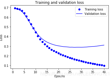

plt.clf()   # 清除数字
plt.plot(epochs, acc, 'bo', label='Training acc')
plt.plot(epochs, val_acc, 'b', label='Validation acc')
plt.title('Training and validation accuracy')
plt.xlabel('Epochs')
plt.ylabel('Accuracy')
plt.legend()
plt.show()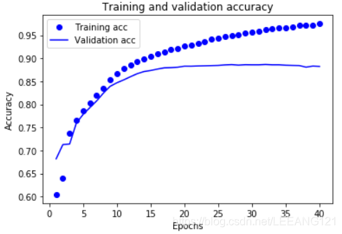

In the figure, the representative point value train loss (Loss) and accuracy (Accuracy), the solid line represents the value of loss verification (Loss) and accuracy (accuracy).

Note that the loss of value of training with each epoch trained decline in accuracy (accuracy) with each epoch rise. When used in a gradient descent optimization is to be expected - in each iteration should minimize the expected value.

The expense of the value of the verification process (loss) and accuracy (accuracy) is not the case - they seem to reach a peak after 20 epoch. This is an example of over-fitting: model performance on the training data to be better than the performance of the data had never seen before of. After that, the model over-optimization study and represent specific training data, not the data can be generalized to the test.

For this particular case, we can stop the train after about 20 epoch to avoid over-fitting.

to sum up

For the network architecture keras depth study, the main divided into the following steps:
1. load data
2, data preprocessing
3, define the model
4, compile model
5, training model
6, evaluation model
7, the predicted
8, save model
for how to save the model, how will the trained models directly brought to our own data to predict, I will be described in other sections.