Dossier d'apprentissage : Vesuvius Challenge : Tutoriel sur la détection d'encre

Vesuvius Challenge : Tutoriel sur la détection d'encre Vesuvius Challenge : Tutoriel sur la détection d'encre

1. Jetez un oeil à l'image

Initialisez certaines variables, affichez des photos de fragments. Mais ça marche. Il s’agit d’une photo infrarouge car l’encre est plus facile à voir sous la lumière infrarouge.

import torch
import torch.nn as nn
import torch.optim as optim
import numpy as np
import glob
import PIL.Image as Image
import torch.utils.data as data
import matplotlib.pyplot as plt
import matplotlib.patches as patches
from tqdm import tqdm
from ipywidgets import interact, fixed

PREFIX = '/kaggle/input/vesuvius-challenge/train/1/'
BUFFER = 30  # Buffer size in x and y direction 表示在 x 和 y 方向上的缓存区大小为 30
Z_START = 27 # First slice in the z direction to use 表示在 z 方向上第一个用到的切片数量，从第 27 个切片开始
Z_DIM = 10   # Number of slices in the z direction 表示在 z 方向上需要用到的切片数量，即选取 10 个切片进行处理
TRAINING_STEPS = 30000 #迭代次数
LEARNING_RATE = 0.03 #初始学习率
BATCH_SIZE = 32 #batchsize
DEVICE = torch.device("cuda" if torch.cuda.is_available() else "cpu")

plt.imshow(Image.open(PREFIX+"ir.png"), cmap="gray")

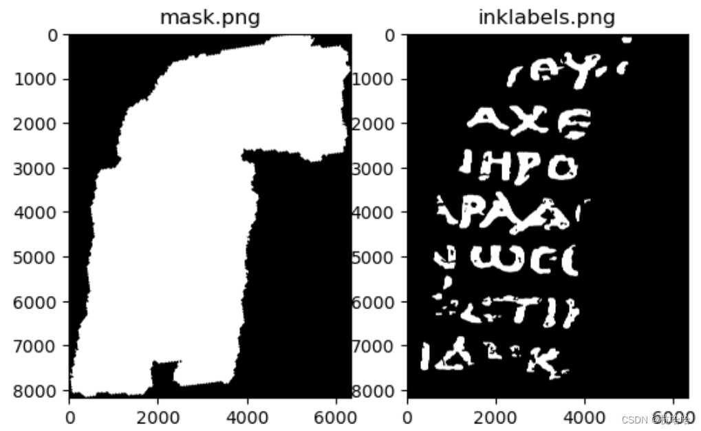
2. Chargez les étiquettes et les masques :

mask.png : Un masque de pixels contenant des données et quels pixels doivent être ignorés.

inklabels.png : Nos données d'étiquette : si un pixel contient ou non de l'encre (celle-ci est étiquetée à la main sur la base de photos infrarouges).

mask = np.array(Image.open(PREFIX+"mask.png").convert('1'))
label = torch.from_numpy(np.array(Image.open(PREFIX+"inklabels.png"))).gt(0).float().to(DEVICE)
fig, (ax1, ax2) = plt.subplots(1, 2)
ax1.set_title("mask.png")
ax1.imshow(mask, cmap='gray')
ax2.set_title("inklabels.png")
ax2.imshow(label.cpu(), cmap='gray')
plt.show()

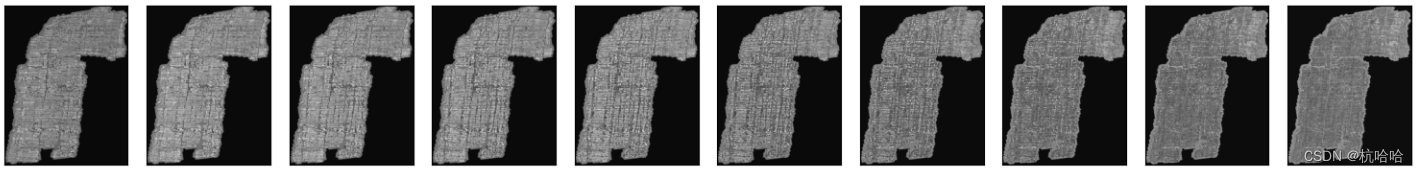
3. Chargez l'image radiographique 3D de la feuille de papyrus

Cette image est représentée comme une pile d'images .tif. La pile d'images est une série de tableaux d'images en niveaux de gris de 16 bits, chacune représentant une « tranche » le long de l'axe z, du bas vers le dessus du papyrus. Nous allons le convertir en un tenseur 4D avec un type de données float 32 bits et convertir les valeurs de pixels dans la plage [0, 1].
Pour économiser de la mémoire, seules certaines tranches internes (tranches Z_DIM) sont chargées. Voir l'image.

images = [np.array(Image.open(filename), dtype=np.float32)/65535.0 for filename in tqdm(sorted(glob.glob(PREFIX+"surface_volume/*.tif"))[Z_START:Z_START+Z_DIM])]
image_stack = torch.stack([torch.from_numpy(image) for image in images], dim=0).to(DEVICE)

fig, axes = plt.subplots(1, len(images), figsize=(15, 3))
for image, ax in zip(images, axes):
  ax.imshow(np.array(Image.fromarray(image).resize((image.shape[1]//20, image.shape[0]//20)), dtype=np.float32), cmap='gray')
  ax.set_xticks([]); ax.set_yticks([])
fig.tight_layout()
plt.show()

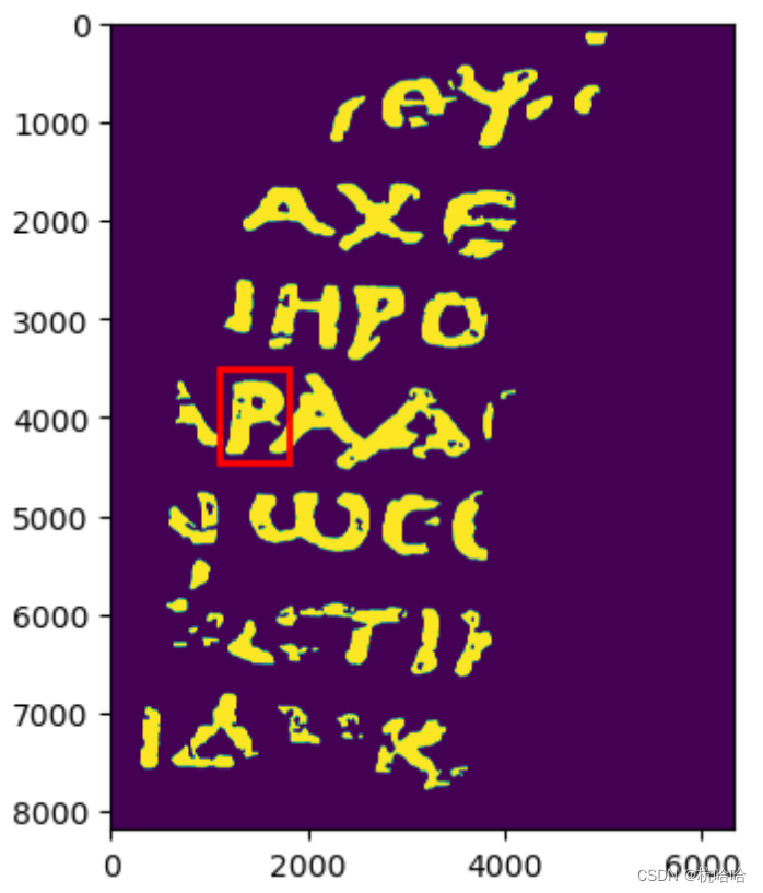
4 Créer un ensemble de données de sous-volume

Utilisez un petit rectangle autour de la lettre « P » pour l'évaluation et excluez ces pixels de l'ensemble d'apprentissage. (En fait, c'est une lettre grecque « rho » qui ressemble à notre « P ».)

rect = (1100, 3500, 700, 950)
fig, ax = plt.subplots()
ax.imshow(label.cpu())
patch = patches.Rectangle((rect[0], rect[1]), rect[2], rect[3], linewidth=2, edgecolor='r', facecolor='none')
ax.add_patch(patch)
plt.show()

5. Définissez un ensemble de données PyTorch et un modèle simple et entraînez-le.

class SubvolumeDataset(data.Dataset):
    def __init__(self, image_stack, label, pixels):
        self.image_stack = image_stack
        self.label = label
        self.pixels = pixels
    def __len__(self):
        return len(self.pixels)
    def __getitem__(self, index):
        y, x = self.pixels[index]
        subvolume = self.image_stack[:, y-BUFFER:y+BUFFER+1, x-BUFFER:x+BUFFER+1].view(1, Z_DIM, BUFFER*2+1, BUFFER*2+1)
        inklabel = self.label[y, x].view(1)
        return subvolume, inklabel

model = nn.Sequential(
    nn.Conv3d(1, 16, 3, 1, 1), nn.MaxPool3d(2, 2),
    nn.Conv3d(16, 32, 3, 1, 1), nn.MaxPool3d(2, 2),
    nn.Conv3d(32, 64, 3, 1, 1), nn.MaxPool3d(2, 2),
    nn.Flatten(start_dim=1),
    nn.LazyLinear(128), nn.ReLU(),
    nn.LazyLinear(1), nn.Sigmoid()
).to(DEVICE)

print("Generating pixel lists...")
# Split our dataset into train and val. The pixels inside the rect are the 
# val set, and the pixels outside the rect are the train set.
# Adapted from https://www.kaggle.com/code/jamesdavey/100x-faster-pixel-coordinate-generator-1s-runtime
# Create a Boolean array of the same shape as the bitmask, initially all True
not_border = np.zeros(mask.shape, dtype=bool)
not_border[BUFFER:mask.shape[0]-BUFFER, BUFFER:mask.shape[1]-BUFFER] = True
arr_mask = np.array(mask) * not_border
inside_rect = np.zeros(mask.shape, dtype=bool) * arr_mask
# Sets all indexes with inside_rect array to True
inside_rect[rect[1]:rect[1]+rect[3]+1, rect[0]:rect[0]+rect[2]+1] = True
# Set the pixels within the inside_rect to False
outside_rect = np.ones(mask.shape, dtype=bool) * arr_mask
outside_rect[rect[1]:rect[1]+rect[3]+1, rect[0]:rect[0]+rect[2]+1] = False
pixels_inside_rect = np.argwhere(inside_rect)
pixels_outside_rect = np.argwhere(outside_rect)

print("Training...")
train_dataset = SubvolumeDataset(image_stack, label, pixels_outside_rect)
train_loader = data.DataLoader(train_dataset, batch_size=BATCH_SIZE, shuffle=True)
criterion = nn.BCELoss()
optimizer = optim.SGD(model.parameters(), lr=LEARNING_RATE)
scheduler = torch.optim.lr_scheduler.OneCycleLR(optimizer, max_lr=LEARNING_RATE, total_steps=TRAINING_STEPS)
model.train()
# running_loss = 0.0
for i, (subvolumes, inklabels) in tqdm(enumerate(train_loader), total=TRAINING_STEPS):
    if i >= TRAINING_STEPS:
        break
    optimizer.zero_grad()
    outputs = model(subvolumes.to(DEVICE))
    loss = criterion(outputs, inklabels.to(DEVICE))
    loss.backward()
    optimizer.step()
    scheduler.step()

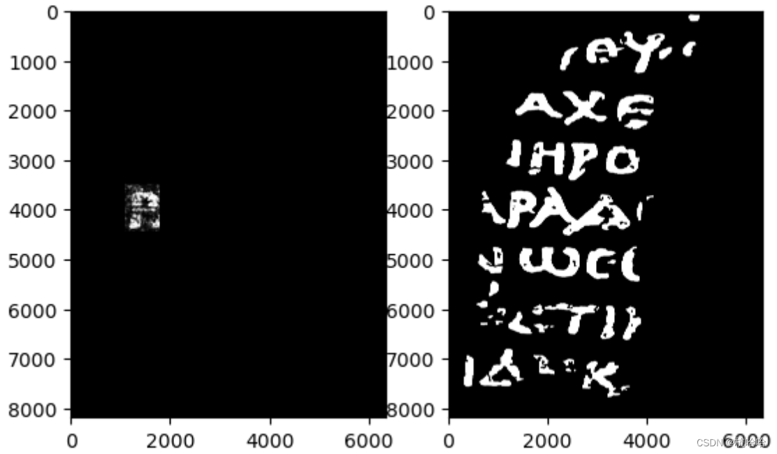
6. Vérifiez simplement

eval_dataset = SubvolumeDataset(image_stack, label, pixels_inside_rect)
eval_loader = data.DataLoader(eval_dataset, batch_size=BATCH_SIZE, shuffle=False)
output = torch.zeros_like(label).float()
model.eval()
with torch.no_grad():
    for i, (subvolumes, _) in enumerate(tqdm(eval_loader)):
        for j, value in enumerate(model(subvolumes.to(DEVICE))):
            output[tuple(pixels_inside_rect[i*BATCH_SIZE+j])] = value

fig, (ax1, ax2) = plt.subplots(1, 2)
ax1.imshow(output.cpu(), cmap='gray')
ax2.imshow(label.cpu(), cmap='gray')
plt.show()

7. Choisissez un seuil, un niveau de confiance de 0,4.

THRESHOLD = 0.4
fig, (ax1, ax2) = plt.subplots(1, 2)
ax1.imshow(output.gt(THRESHOLD).cpu(), cmap='gray')
ax2.imshow(label.cpu(), cmap='gray')
plt.show()

8. Générer un fichier csv

Enfin, Kaggle attend un fichier submit.csv codé en longueur et le génère.

# Adapted from https://www.kaggle.com/code/stainsby/fast-tested-rle/notebook
# and https://www.kaggle.com/code/kotaiizuka/faster-rle/notebook
def rle(output):
    pixels = np.where(output.flatten().cpu() > THRESHOLD, 1, 0).astype(np.uint8)
    pixels[0] = 0
    pixels[-1] = 0
    runs = np.where(pixels[1:] != pixels[:-1])[0] + 2
    runs[1::2] = runs[1::2] - runs[:-1:2]
    return ' '.join(str(x) for x in runs)
rle_output = rle(output)
# This doesn't make too much sense, but let's just output in the required format
# so notebook works as a submission. :-)
print("Id,Predicted\na," + rle_output + "\nb," + rle_output, file=open('submission.csv', 'w'))