用python绘制曼彻斯特编码等八种常见数据编码方式的波形图

用python绘制八种数据编码方式的波形图

---

2020春季北京航空航天大学计算机学院物联网引论课程作业，介绍八种常见数据编码方式并实践画出波形图。本文使用了python中的二维图像模块matplotlib。博主在信号与通信原理方面功底不深，如有表达不准或错误敬请指出。

---

物联网或通信领域有许多种常用的数据编码方式，这些编码方式在不同的通信机制下能够分别发挥优势帮助我们进行数据传输。本文用示例讨论以下八种数据编码方式，并使用python绘制相应的波形图：

• 反向不归零码（Non Return to Zero）
• 曼彻斯特编码（Manchester）
• 单极性归零编码（Unipolar RZ）
• 差动双相编码（DBP）
• 米勒编码（Miller）
• 差动编码（Differential）
• 脉冲宽度编码（Pulse Width Modulation）
• 脉冲位置编码（Pulse Position Modulation）
  
  

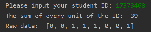
例如，我们要对一组八位十进制的学号进行编码，压缩的方式假设为：学号各个十进制位相加，得到一个两位十进制数，将这两位十进制数直接看作两位十六进制数（例如直接将27看作0x27），然后将这两位16进制数转化为8位二进制比特，进行传输（这一过程是课程组作业给出的，仅作示意即可，不必细究）：

student_id = input('Please input your student ID: ')
id_sum = 0
for unit in student_id:
    id_sum += int(unit)
raw_data_str = bin((id_sum % 10) + ((id_sum // 10) % 10) * 16)
raw_data_str = raw_data_str[2:].rjust(8, '0')
for bit in raw_data_str:
    raw_data.append(int(bit))

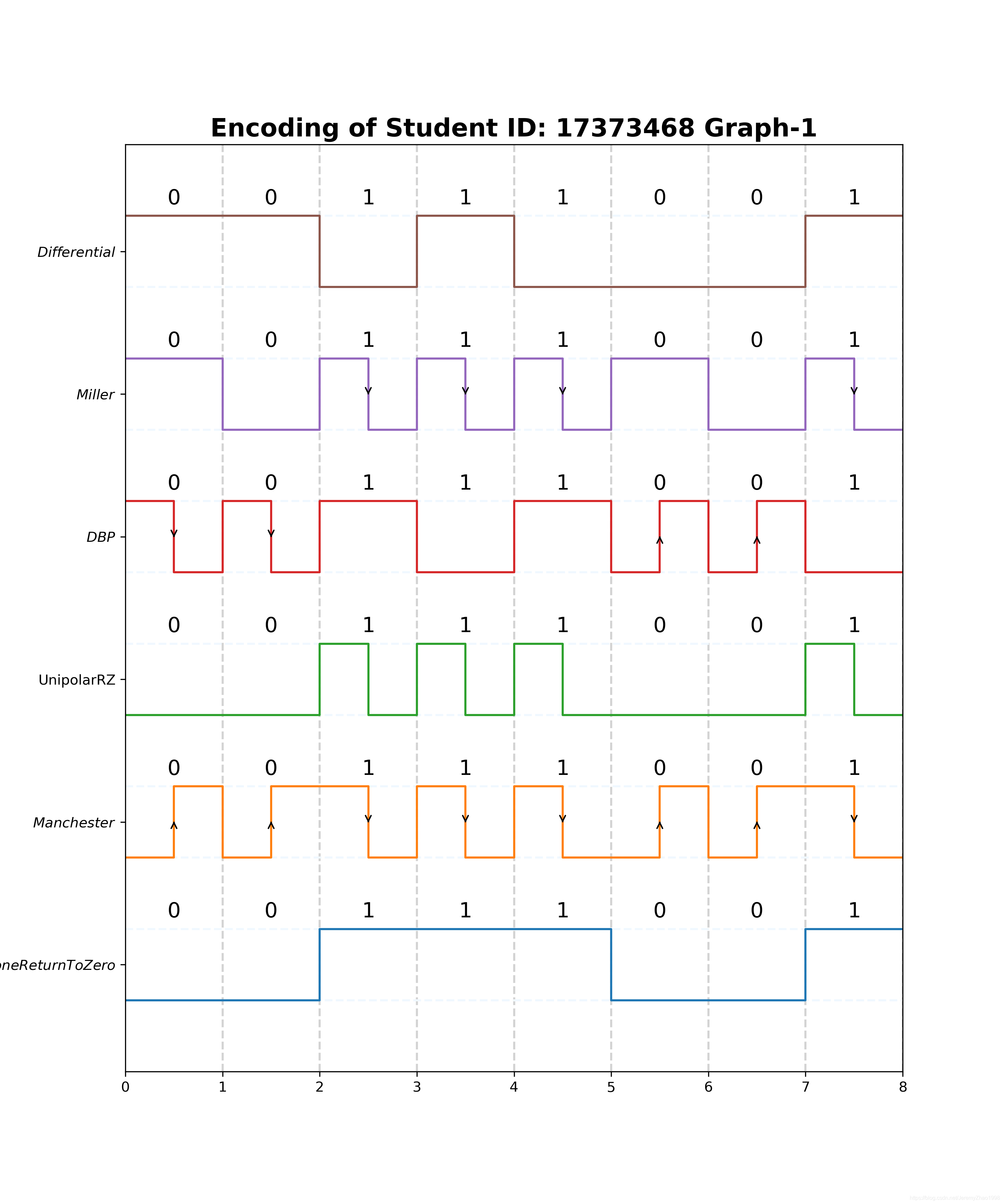
我们使用matplotlib来绘制二维波形图，首先import该模块，以及做一些初始化坐标轴和标识的工作。由于不同的编码方式传送同一段比特流所用的周期数不同，我们用两张图来容纳八种编码波形图：

import matplotlib.pyplot as plt

def settings_1():
    plt.figure(figsize=(10, 12))
    plt.rcParams['savefig.dpi'] = 300
    plt.rcParams['figure.dpi'] = 300
    plt.title('Encoding of Student ID: ' + student_id + ' Graph-1',
              fontsize=18, fontweight='bold')
    plt.xlim((0, 8))
    plt.ylim((-1, 12))
    plt.yticks([0.5, 2.5, 4.5, 6.5, 8.5, 10.5],
               [r'$NoneReturnToZero$', r'$Manchester$', r'UnipolarRZ', r'$DBP$',
                r'$Miller$', r'$Differential$'])
    for i in range(8):
        plt.plot([i+1, i+1], [-1, 16], color="lightgrey", linestyle="--")
    for i in range(12):
        plt.plot([0, 8], [i, i], color="aliceblue", linestyle="--")
    for i in range(6):
        for j in range(8):
            plt.text(j + 0.5, i * 2 + 1.1, str(raw_data[j]), fontsize=15,
                     verticalalignment="bottom", horizontalalignment="center")

def settings_2():
    plt.figure(figsize=(18, 5))
    plt.rcParams['savefig.dpi'] = 300
    plt.rcParams['figure.dpi'] = 300
    plt.title('Encoding of Student ID: ' + student_id + ' Graph-2',
              fontsize=18, fontweight='bold')
    plt.xlim((0, 16))
    plt.ylim((-1, 4))
    plt.yticks([0.5, 2.5], [r'$PulseWidthModulation$', r'$PulsePositionModulation$'])
    for i in range(16):
        plt.plot([i + 1, i + 1], [-1, 4], color="lightgrey", linestyle="--")
    for i in range(4):
        plt.plot([0, 16], [i, i], color="aliceblue", linestyle="--")

---

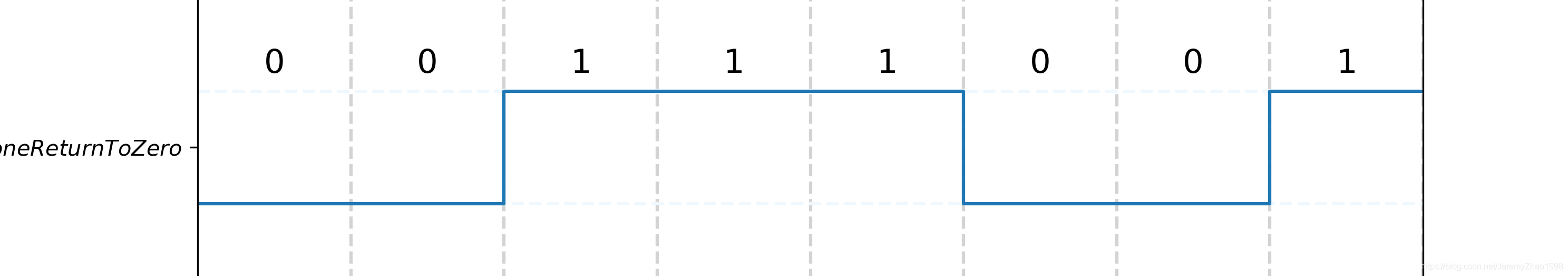
反向不归零码（Non Return to Zero）

最简单的编码方式，简单地用高电平表示1，低电平表示0。需要在此说明的是，x_standard列表是为了在多个函数中共享，设计成了全局变量（由于多种编码方式都是在一个周期内对四个点进行连接形成方波，因此这些点的横坐标都是相同的）。函数参数low和high分别是低电平和高电平在图中的纵坐标，由main函数传入。matplotlib最终显示图像的plt.show()在main函数进行调用。这些说明在后面几个编码函数中不再重复提起。

x_standard = []
for i_standard in range(8):
    x_standard.append(i_standard)
    x_standard.append(i_standard + 0.5)
    x_standard.append(i_standard + 0.5)
    x_standard.append(i_standard + 1)

def none_return_to_zero(low, high):
    y = []
    y_cycle = ([low, low, low, low], [high, high, high, high])
    for i in range(8):
        y.extend(y_cycle[raw_data[i]])
    plt.plot(x_standard, y)

---

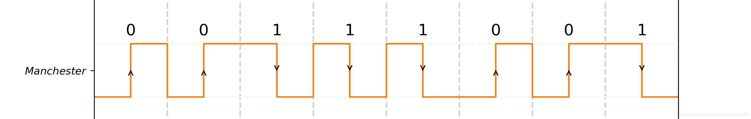
曼彻斯特编码（Manchester）

曼彻斯特编码将高低电平判断改为正负跳变判断，由高电平向低电平的负跳变表示1，低电平向高电平的正跳变表示0。这样做的好处在于跳变和模糊的“高低”电平相比更容易检测，避免了电压不稳造成的“中”电平无法判断的问题。代码中为正负跳变加了相应的箭头指示方向。

def manchester(low, high):
    y = []
    for i in range(8):
        if raw_data[i] == 0:
            y.extend([low, low, high, high])
            plt.annotate("", xy=(i + 0.5, low + 0.51), xytext=(i + 0.5, low + 0.49),
                         arrowprops=dict(arrowstyle="->", connectionstyle="arc3"))
        elif raw_data[i] == 1:
            y.extend([high, high, low, low])
            plt.annotate("", xy=(i + 0.5, low + 0.49), xytext=(i + 0.5, low + 0.51),
                         arrowprops=dict(arrowstyle="->", connectionstyle="arc3"))
    plt.plot(x_standard, y)

---

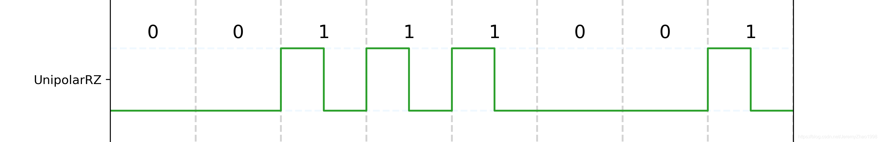
单极性归零编码（Unipolar RZ）

单极性归零编码相对于最简单的反向不归零编码，是让表示1的高电平只在前半周期维持高电平，而后半周期回归低电平，表示0则还是整周期低电平。单极性归零码的主要优点是可以直接提取同步信号，因此单极性归零码常常用作其他码型提取同步信号时的过渡码型，也就是说其他适合信道传输但不能直接提取同步信号的码型，可先变换为单极性归零码，然后再提取同步信号。

def unipolar_rz(low, high):
    y = []
    y_cycle = ([low, low, low, low], [high, high, low, low])
    for i in range(8):
        y.extend(y_cycle[raw_data[i]])
    plt.plot(x_standard, y)

---

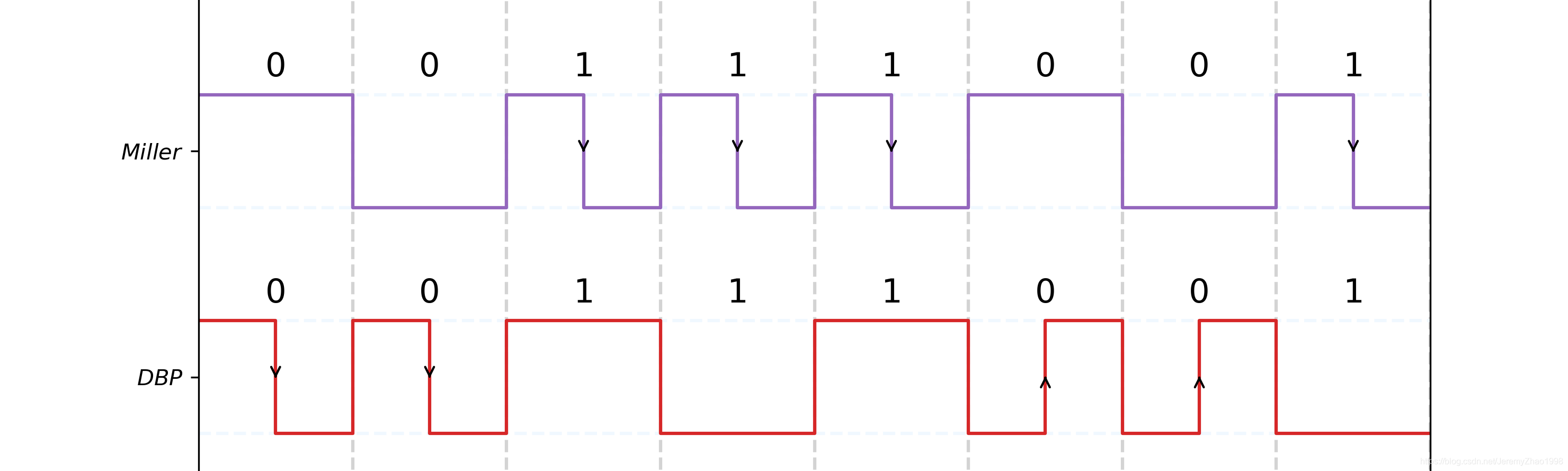
差动双相编码（DBP）与米勒编码（Miller）

差动双相编码是通过在一个位周期内采用电平变化来表示逻辑0和1的。如果电平只在一个位周期的起始处发生跳变（逻辑电平的翻转1—>0 / 0—>1）则表示逻辑1，如果电平除了在一个位周期的起始处发生跳变，还在位周期的中间发生跳变，则表示逻辑0。

而米勒编码与差动双相编码恰好相反，除起始位置之外在周期中间也发生跳变表示1，否则表示0。差动双相编码和米勒编码让任意的跳变都表示数据。

米勒编码有一种变形，是将所有的跳变都用负脉冲替代，其他地方均为高电平。这样一来只需要检测脉冲的位置即可。

def dbp_miller(low_high, coding):
    y = []
    p = 1
    jump = 0
    if coding == 'miller':
        jump = 1
    for i in range(8):
        if raw_data[i] == jump:
            y.extend([low_high[p], low_high[p]])
            if p == 0:
                plt.annotate("", xy=(i + 0.5, low_high[0] + 0.51), 
                             xytext=(i + 0.5, low_high[0] + 0.49),
                             arrowprops=dict(arrowstyle="->",
                                             connectionstyle="arc3"))
            elif p == 1:
                plt.annotate("", xy=(i + 0.5, low_high[0] + 0.49), 
                             xytext=(i + 0.5, low_high[0] + 0.51),
                             arrowprops=dict(arrowstyle="->", 
                                             connectionstyle="arc3"))
            p = (p + 1) % 2
            y.extend([low_high[p], low_high[p]])
        else:
            y.extend([low_high[p], low_high[p], low_high[p], low_high[p]])
        p = (p + 1) % 2
    plt.plot(x_standard, y)

---

差动编码（Differential）

差动编码仅在周期开始处产生跳变，高电平时跳变，低电平时保持不变。

def differential(low, high):
    y = []
    y_cycle = ([low, low, low, low], [high, high, high, high])
    p = 1
    for i in range(8):
        if raw_data[i] == 1:
            p = (p + 1) % 2
        y.extend(y_cycle[p])
    plt.plot(x_standard, y)

---

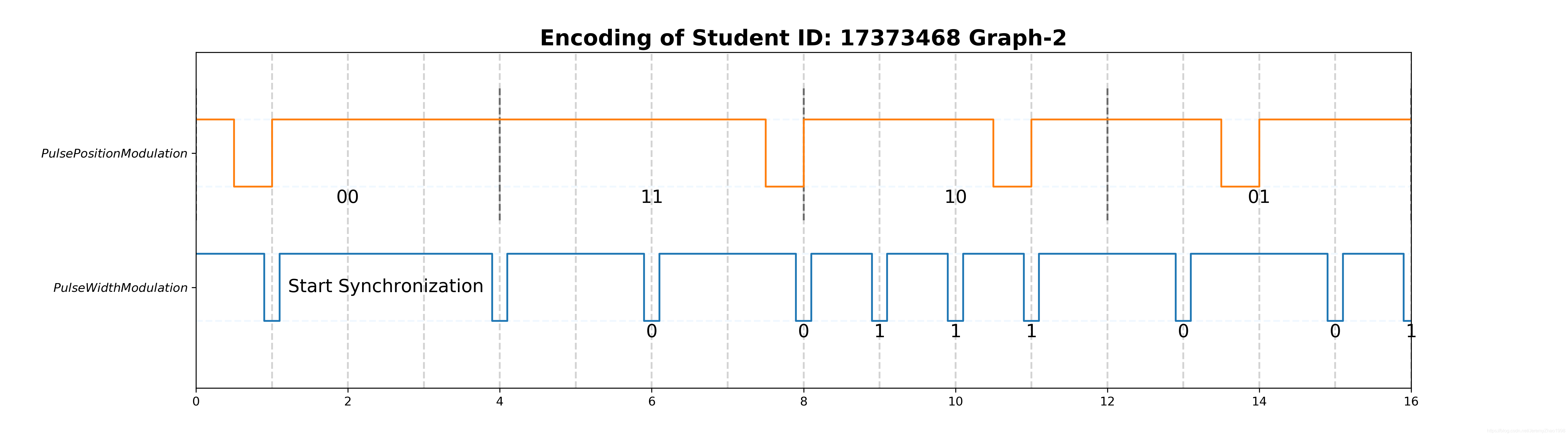
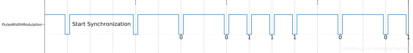
脉冲宽度编码（Pulse Width Modulation）

脉冲宽度编码也称脉冲间歇编码，他利用脉冲来“截断”信号，将信号截成两个周期表示0，截成一个周期表示1。“开始”和“同步”也使用不同的脉冲间隔来表示，本文的示意图中直接采用三个周期表示“开始”和“同步”，示意即可。利用脉冲间隔编码，其所需要的周期数不仅与数据大小有关，并且与传输的数据内容有关。

def pulse_width_modulation(low, high):
    x = [0.00, 0.90, 0.9, 1.1, 1.10, 3.90, 3.9, 4.1]
    y = [high, high, low, low, high, high, low, low]
    plt.text(2.5, low + 0.5, 'Start Synchronization', fontsize=15,
             verticalalignment="center", horizontalalignment="center")
    t = 4.1
    for i in range(8):
        y.extend([high, high, low, low])
        width = 1.8
        if raw_data[i] == 1:
            width = 0.8
        x.append(t)
        t += width
        x.append(t)
        x.append(t)
        plt.text(t + 0.1, low - 0.3, str(raw_data[i]), fontsize=15,
                 verticalalignment="bottom", horizontalalignment="center")
        t += 0.2
        x.append(t)
    plt.plot(x, y)

---

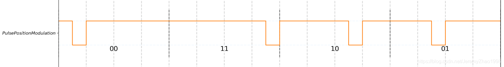
脉冲位置编码（Pulse Position Modulation）

脉冲位置编码相当于独热码，根据脉冲的位置来确定数据。例如要表示两位二进制数，那么每四个周期只需要发送一个脉冲，根据脉冲的位置就可以确定这个两位二进制数。本文的代码中也采用将16位二进制数每两位发送。

def pulse_position_modulation(low, high):
    x, y = [], []
    t = 0
    for i in range(4):
        y.extend([high, high, low, low, high, high])
        width = raw_data[i * 2] * 2 + raw_data[i * 2 + 1] + 0.5
        plt.plot([t, t], [low - 0.5, high + 0.5], color="dimgray", linestyle="--")
        x.append(t)
        t += width
        x.append(t)
        x.append(t)
        t += 0.5
        x.append(t)
        x.append(t)
        t += (3.5 - width)
        x.append(t)
        plt.plot([t, t], [low - 0.5, high + 0.5], color="dimgray", linestyle="--")
        plt.text(t - 2, low - 0.3, str(raw_data[i * 2]) + str(raw_data[i * 2 + 1]),
                 fontsize=15, verticalalignment="bottom", 
                 horizontalalignment="center")
    plt.plot(x, y)

---

最终在main函数中调用各个函数，画出完整的图形。完整的代码如下：

# -*- coding: utf-8 -*-
# @Time       : 2020/3/16 16:07
# @Author     : JeremyZhao1998
# @File       : data_coding.py
# @Software   : PyCharm
# @Description: To demonstrate different encodings by drawing waveforms.
import matplotlib.pyplot as plt

student_id = input('Please input your student ID: ')
raw_data = []
x_standard = []
for i_standard in range(8):
    x_standard.append(i_standard)
    x_standard.append(i_standard + 0.5)
    x_standard.append(i_standard + 0.5)
    x_standard.append(i_standard + 1)


def settings_1():
    plt.figure(figsize=(10, 12))
    plt.rcParams['savefig.dpi'] = 300
    plt.rcParams['figure.dpi'] = 300
    plt.title('Encoding of Student ID: ' + student_id + ' Graph-1',
              fontsize=18, fontweight='bold')
    plt.xlim((0, 8))
    plt.ylim((-1, 12))
    plt.yticks([0.5, 2.5, 4.5, 6.5, 8.5, 10.5],
               [r'$NoneReturnToZero$', r'$Manchester$', r'UnipolarRZ', r'$DBP$',
                r'$Miller$', r'$Differential$'])
    for i in range(8):
        plt.plot([i+1, i+1], [-1, 16], color="lightgrey", linestyle="--")
    for i in range(12):
        plt.plot([0, 8], [i, i], color="aliceblue", linestyle="--")
    for i in range(6):
        for j in range(8):
            plt.text(j + 0.5, i * 2 + 1.1, str(raw_data[j]), fontsize=15,
                     verticalalignment="bottom", horizontalalignment="center")


def settings_2():
    plt.figure(figsize=(18, 5))
    plt.rcParams['savefig.dpi'] = 300
    plt.rcParams['figure.dpi'] = 300
    plt.title('Encoding of Student ID: ' + student_id + ' Graph-2',
              fontsize=18, fontweight='bold')
    plt.xlim((0, 16))
    plt.ylim((-1, 4))
    plt.yticks([0.5, 2.5], [r'$PulseWidthModulation$', 
                            r'$PulsePositionModulation$'])
    for i in range(16):
        plt.plot([i + 1, i + 1], [-1, 4], color="lightgrey", linestyle="--")
    for i in range(4):
        plt.plot([0, 16], [i, i], color="aliceblue", linestyle="--")


def none_return_to_zero(low, high):
    y = []
    y_cycle = ([low, low, low, low], [high, high, high, high])
    for i in range(8):
        y.extend(y_cycle[raw_data[i]])
    plt.plot(x_standard, y)


def manchester(low, high):
    y = []
    for i in range(8):
        if raw_data[i] == 0:
            y.extend([low, low, high, high])
            plt.annotate("", xy=(i + 0.5, low + 0.51), xytext=(i + 0.5, low + 0.49),
                         arrowprops=dict(arrowstyle="->", connectionstyle="arc3"))
        elif raw_data[i] == 1:
            y.extend([high, high, low, low])
            plt.annotate("", xy=(i + 0.5, low + 0.49), xytext=(i + 0.5, low + 0.51),
                         arrowprops=dict(arrowstyle="->", connectionstyle="arc3"))
    plt.plot(x_standard, y)


def unipolar_rz(low, high):
    y = []
    y_cycle = ([low, low, low, low], [high, high, low, low])
    for i in range(8):
        y.extend(y_cycle[raw_data[i]])
    plt.plot(x_standard, y)


def dbp_miller(low_high, coding):
    y = []
    p = 1
    jump = 0
    if coding == 'miller':
        jump = 1
    for i in range(8):
        if raw_data[i] == jump:
            y.extend([low_high[p], low_high[p]])
            if p == 0:
                plt.annotate("", xy=(i + 0.5, low_high[0] + 0.51), 
                             xytext=(i + 0.5, low_high[0] + 0.49),
                             arrowprops=dict(arrowstyle="->", 
                                             connectionstyle="arc3"))
            elif p == 1:
                plt.annotate("", xy=(i + 0.5, low_high[0] + 0.49), 
                             xytext=(i + 0.5, low_high[0] + 0.51),
                             arrowprops=dict(arrowstyle="->", 
                                             connectionstyle="arc3"))
            p = (p + 1) % 2
            y.extend([low_high[p], low_high[p]])
        else:
            y.extend([low_high[p], low_high[p], low_high[p], low_high[p]])
        p = (p + 1) % 2
    plt.plot(x_standard, y)


def differential(low, high):
    y = []
    y_cycle = ([low, low, low, low], [high, high, high, high])
    p = 1
    for i in range(8):
        if raw_data[i] == 1:
            p = (p + 1) % 2
        y.extend(y_cycle[p])
    plt.plot(x_standard, y)


def pulse_width_modulation(low, high):
    x = [0.00, 0.90, 0.9, 1.1, 1.10, 3.90, 3.9, 4.1]
    y = [high, high, low, low, high, high, low, low]
    plt.text(2.5, low + 0.5, 'Start Synchronization', fontsize=15,
             verticalalignment="center", horizontalalignment="center")
    t = 4.1
    for i in range(8):
        y.extend([high, high, low, low])
        width = 1.8
        if raw_data[i] == 1:
            width = 0.8
        x.append(t)
        t += width
        x.append(t)
        x.append(t)
        plt.text(t + 0.1, low - 0.3, str(raw_data[i]), fontsize=15,
                 verticalalignment="bottom", horizontalalignment="center")
        t += 0.2
        x.append(t)
    plt.plot(x, y)


def pulse_position_modulation(low, high):
    x, y = [], []
    t = 0
    for i in range(4):
        y.extend([high, high, low, low, high, high])
        width = raw_data[i * 2] * 2 + raw_data[i * 2 + 1] + 0.5
        plt.plot([t, t], [low - 0.5, high + 0.5], color="dimgray", linestyle="--")
        x.append(t)
        t += width
        x.append(t)
        x.append(t)
        t += 0.5
        x.append(t)
        x.append(t)
        t += (3.5 - width)
        x.append(t)
        plt.plot([t, t], [low - 0.5, high + 0.5], color="dimgray", linestyle="--")
        plt.text(t - 2, low - 0.3, str(raw_data[i * 2]) + str(raw_data[i * 2 + 1]),
                 fontsize=15, verticalalignment="bottom", 
                 horizontalalignment="center")
    plt.plot(x, y)


def input_process():
    id_sum = 0
    for unit in student_id:
        id_sum += int(unit)
    print('The sum of every unit of the ID: ', id_sum)
    raw_data_str = bin((id_sum % 10) + ((id_sum // 10) % 10) * 16)
    raw_data_str = raw_data_str[2:].rjust(8, '0')
    for bit in raw_data_str:
        raw_data.append(int(bit))
    print('Raw data: ', raw_data)


if __name__ == '__main__':
    input_process()

    settings_1()
    none_return_to_zero(0, 1)
    manchester(2, 3)
    unipolar_rz(4, 5)
    dbp_miller([6, 7], 'dbp')
    dbp_miller([8, 9], 'miller')
    differential(10, 11)
    plt.savefig('graph-1.png')
    plt.show()

    settings_2()
    pulse_width_modulation(0, 1)
    pulse_position_modulation(2, 3)
    plt.savefig('graph-2.png')
    plt.show()
    print('done')

运行结果如下：