本文介绍了如何在以TF2.1为后端的Keras中搭建多层感知器模型实现序列预测。模型包括一元感知器模型,多元感知器模型,多时间步感知器模型,多变量多时间步感知器模型。
多层感知器,简称MLPs,可用于时间序列预测。使用MLPs进行时间序列预测的挑战在于数据的准备。具体来说,先前的时间步的值在输入时必须展平为特征向量。本文介绍了如何为一系列标准时间序列预测问题编写多层感知器模型。
在深度学习方法应用于时间序列预测中,最热的研究是使用CNN,LSTM和混合模型。这些会在之后的文章中介绍。
文章目录
思维导图
本文内容较多,大概21000字(包含代码),如果之前没有相关基础,比较容易混淆。注意不同的数据构建方式,代码都有细微差别。如果看着比较费劲,可以先看看思维导图,理清思路,本文结构也大体如下。

1. 数据准备
在对单变量序列进行建模之前,必须先进行准备。 MLP模型将学习将过去的观测序列作为输入映射到输出观测的函数。因此,必须将观察序列转换成可以从中学习模型的多个样本。假设有如下单变量序列:
[10, 20, 30, 40, 50, 60, 70, 80, 90]
我们可以将序列分为多个称为样本的输入/输出模式,其中三个时间步长用作输入,一个时间步长用作输出,用于单步预测。
X,  		 y
10, 20, 30,  40
20, 30, 40,  50
30, 40, 50,  60
...
下面的 split_sequence() 函数实现了此功能,将给定的单变量序列拆分为多个样本,其中每个样本具有指定数量的时间步长,而输出为单个时间步长。
import numpy as np

def split_sequence(sequence, sliding_window_width):
    X, y = [], []
    for i in range(len(sequence)):
        # 找到最后一次滑动所截取数据中最后一个元素的索引,
        # 如果这个索引超过原序列中元素的索引则不截取;
        end_element_index = i + sliding_window_width
        if end_element_index > len(sequence) - 1: # 序列中最后一个元素的索引
            break
        sequence_x, sequence_y = sequence[i:end_element_index], sequence[end_element_index] # 取最后一个元素作为预测值y
        X.append(sequence_x)
        y.append(sequence_y)

    #return X,y
    return np.array(X), np.array(y)

if __name__ == '__main__':
    seq_test = [10,20,30,40,50,60,70,80,90]
    sw_width = 3
    seq_test_x, seq_test_y = split_sequence(seq_test, sw_width)
    print(seq_test_x.shape,seq_test_y.shape)
    for i in zip(seq_test_x,seq_test_y):
        print(i)
    for i in range(len(seq_test_x)):
        print(seq_test_x[i], seq_test_y[i])
输出:
(6, 3) (6,)
(array([10, 20, 30]), 40)
(array([20, 30, 40]), 50)
(array([30, 40, 50]), 60)
(array([40, 50, 60]), 70)
(array([50, 60, 70]), 80)
(array([60, 70, 80]), 90)
[10 20 30] 40
[20 30 40] 50
[30 40 50] 60
[40 50 60] 70
[50 60 70] 80
[60 70 80] 90
2. 单变量MLP模型
一个简单的MLP模型具有单个隐藏的节点层和一个用于进行预测的输出层。我们可以如下定义用于单变量时间序列预测的MLP。

from tensorflow.keras.models import Sequential
from tensorflow.keras.layers import LSTM, Dense
model = Sequential()
model.add(Dense(100, activation='relu', input_dim=n_steps))
model.add(Dense(1))
model.compile(optimizer='adam', loss='mse')
每个样本的输入维度在第一个隐藏层定义的 input dim 参数中指定。从技术上讲,模型将把每个时间步看作一个单独的特征,而不是单独的时间步。
我们几乎总是有多个样本,因此,模型期望训练数据的输入部分具有维度或形状:[样本,特征]。上一节中的 split_sequence() 函数输出X的形状 [样本,特征] 可用于建模。该模型利用高效的随机梯度下降算法 Adam 进行拟合,使用均方误差(mse)损失函数进行优化。定义了模型之后就可以进行训练。
model.fit(seq_test_x, seq_test_y, epochs=2000, verbose=0)
在模型拟合后,我们可以利用它进行预测。我们可以通过输入[70,80,90]来预测序列中的下一个值。并期望模型预测输出能接近100。该模型期望输入形状是二维的,具有 [samples,features],因此,在进行预测之前,必须重塑单个输入样本,例如,可以将1个样本和3个时间步作为输入特征,重塑为[1,3]的二维数组。
x_input = np.array([70, 80, 90])
x_input = x_input.reshape((1, sw_width))
yhat = model.predict(x_input, verbose=0)
print(yhat)
输出:
[[101.17381]]
3. 多变量MLP模型
多元时间序列数据是指每一时间步有多个观测值的数据,即有多个特征。对于多变量时间序列数据,常用的有两种主要模型:
- 多输入序列;
- 多个平行系列;
3.1 多输入序列(Multiple Input Series)
一个问题可能有两个或多个并行输入时间序列和一个依赖于输入时间序列的输出时间序列。输入时间序列是平行的,因为每个序列在同一时间步上都有一个观测值。我们可以通过两个并行输入时间序列的简单示例来演示这一点,其中输出序列是输入序列的简单相加。
in_seq1 = np.array([10, 20, 30, 40, 50, 60, 70, 80, 90])
in_seq2 = np.array([15, 25, 35, 45, 55, 65, 75, 85, 95])
out_seq = np.array([in_seq1[i]+in_seq2[i] for i in range(len(in_seq1))])
我们可以将这三个数组重塑为单个数据集,其中每一行是一个时间步,每一列是一个单独的时间序列。这是在CSV文件中存储并行时间序列的标准方法。
# 每一个数组先转换成9×1的二维数组
in_seq1 = in_seq1.reshape((len(in_seq1), 1))
in_seq2 = in_seq2.reshape((len(in_seq2), 1))
out_seq = out_seq.reshape((len(out_seq), 1))
# 使用numpy的hstack方法,沿水平方向堆叠数组,对于二维数组就是沿第二个维度(列)堆叠
dataset = np.hstack((in_seq1, in_seq2, out_seq))
我们看一下dataset:
array([[ 10,  15,  25],
       [ 20,  25,  45],
       [ 30,  35,  65],
       [ 40,  45,  85],
       [ 50,  55, 105],
       [ 60,  65, 125],
       [ 70,  75, 145],
       [ 80,  85, 165],
       [ 90,  95, 185]])
与单变量时间序列一样,我们必须将这些数据构造成具有输入和输出样本的样本。我们需要将数据分成样本,保持两个输入序列的观测顺序。如果我们选择三个输入时间步骤,那么第一个示例将如下所示:
输入:
10, 15
20, 25
30, 35
输出:
65
也就是说,将每个并行序列的前三个时间步作为输入提供给模型,并且在第三个时间步,在本例中为65,模型将其与输出序列中的值相关联。我们可以看到,在将时间序列转换为输入/输出样本以训练模型时,我们将不得不放弃输出时间序列中的一些值,因为在先前的时间步,我们在输入时间序列中没有值。反过来,输入时间步数大小的选择将对训练数据的使用量产生重要影响。我们可以定义一个名为 split_sequences() 的函数来实现数据集划分。
def split_sequences(sequences, sliding_window_width):
    X, y = [], []
    for i in range(len(sequences)):
        # 找到最后一次滑动所截取数据中最后一个元素的索引,
        # 如果这个索引超过原序列中元素的索引则不截取;
        end_element_index = i + sliding_window_width
        if end_element_index > len(sequences) : # 序列中最后一个元素的索引
            break

        # 使用二维数组切片来截取输入数据X和标签y;:-1 表示截取第1,2列数据(共3列);-1表示截取最后一列数据;
        sequence_x, sequence_y = sequences[i:end_element_index ,:-1], sequences[end_element_index-1, -1] # 取最后一个元素作为预测值y
        X.append(sequence_x)
        y.append(sequence_y)

    #return X,y
    return np.array(X), np.array(y)

if __name__ == '__main__':
    sw_width = 3
    X, y = split_sequences(dataset, sw_width)
    print(X.shape, y.shape)
    for i in range(len(X)):
        print(X[i], y[i])
输出:
(7, 3, 2) (7,)
[[10 15]
 [20 25]
 [30 35]] 65
[[20 25]
 [30 35]
 [40 45]] 85
[[30 35]
 [40 45]
 [50 55]] 105
[[40 45]
 [50 55]
 [60 65]] 125
[[50 55]
 [60 65]
 [70 75]] 145
[[60 65]
 [70 75]
 [80 85]] 165
[[70 75]
 [80 85]
 [90 95]] 185
在拟合MLP之前,必须将输入样本的形状变平。MLP要求每个样本的输入部分的形状是一个向量。对于多变量输入,有多个向量,每个时间步一个向量。我们可以展平每个输入样本:
[[10 15]
[20 25]
[30 35]]
展平输入为:
[10, 15, 20, 25, 30, 35]
我们可以计算每个输入向量的长度,即时间步数乘以特征数或时间序列数。然后我们可以使用这个向量大小来重塑输入。
n_input = X.shape[1] * X.shape[2]
X = X.reshape((X.shape[0], n_input))
我们看一下X:
array([[10, 15, 20, 25, 30, 35],
       [20, 25, 30, 35, 40, 45],
       [30, 35, 40, 45, 50, 55],
       [40, 45, 50, 55, 60, 65],
       [50, 55, 60, 65, 70, 75],
       [60, 65, 70, 75, 80, 85],
       [70, 75, 80, 85, 90, 95]])
3.1.1 MLP 模型
现在可以为多元输入定义一个MLP模型,其中向量长度用于输入维参数。
model = Sequential()
model.add(Dense(100, activation='relu', input_dim=n_input))
model.add(Dense(1))
model.compile(optimizer='adam', loss='mse')

model.fit(X, y, epochs=2000, verbose=0)
输入数据做预测:
x_input = np.array([[80, 85], [90, 95], [100, 105]])
x_input = x_input.reshape((1, n_input))
yhat = model.predict(x_input, verbose=0)
print(yhat)
输出:
[[206.24257]]
3.1.2 Multi-headed MLP 模型
还有另一种更精细的方法来模拟这个问题。每个输入序列可以由单独的MLP处理,并且在对输出序列进行预测之前,可以组合这些子模型中的每个的输出。我们可以称之为 Multi-headed MLP模型。它可能提供更多的灵活性或更好的性能,这取决于正在建模的问题的具体情况。这种类型的模型可以使用Keras函数API在Keras中定义。首先,我们可以将第一个输入模型定义为一个MLP,其输入层期望向量具有n步特征。
    visible1 = Input(shape=(sliding_window_width,))
    dense1 = Dense(100, activation='relu')(visible1)
    visible2 = Input(shape=(sliding_window_width,))
    dense2 = Dense(100, activation='relu')(visible2)
定义了两个输入子模型之后,可以将每个模型的输出合并为一个长向量,在对输出序列进行预测之前可以对其进行解释。
    merge = concatenate([dense1, dense2])
    output = Dense(1)(merge)

    model = Model(inputs=[visible1, visible2], outputs=output)
下图提供了该模型的外观示意图,包括每个层的输入和输出的形状。绘图方法请看下文完整代码。
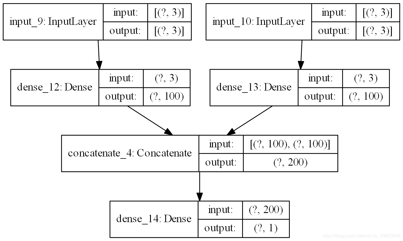
此模型要求将输入作为有两个元素组成的列表提供,其中列表中的每个元素都包含其中一个子模型的数据。为了达到这个目的,我们可以将3D输入数据分割成两个独立的输入数据数组:即从一个形状为[7,3,2]的三维数组转化为两个形状为[7,3]的二维数组。
X1 = X[:, :, 0]
X2 = X[:, :, 1]
转换完成后,可以进行编译,然后训练:
model.compile(optimizer='adam', loss='mse')
model.fit([X1, X2], y, epochs=2000, verbose=0)
同样,在进行一步预测时,我们必须将单个样本的数据准备为两个独立的二维数组。
x_input = array([[80, 85], [90, 95], [100, 105]])
x1 = x_input[:, 0].reshape((1, sw_width))
x2 = x_input[:, 1].reshape((1, sw_width)
进行预测:
yhat = model.predict([x1, x2], verbose=0)
print(yhat)
完整代码:
from tensorflow.keras.models import Model
from tensorflow.keras.layers import Input,Dense,concatenate
from tensorflow.keras.utils import plot_model
import numpy as np

def split_sequences(sequences, sliding_window_width):
    X, y = [], []
    for i in range(len(sequences)):
        # 找到最后一次滑动所截取数据中最后一个元素的索引,
        # 如果这个索引超过原序列中元素的索引则不截取;
        end_element_index = i + sliding_window_width
        if end_element_index > len(sequences) : # 序列中最后一个元素的索引
            break

        # 使用二维数组切片来截取输入数据X和标签y;:-1 表示截取第1,2列数据(共3列);-1表示截取最后一列数据;
        sequence_x, sequence_y = sequences[i:end_element_index ,:-1], sequences[end_element_index-1, -1] # 取最后一个元素作为预测值y
        X.append(sequence_x)
        y.append(sequence_y)

    #return X,y
    return np.array(X), np.array(y)

def multiple_input_series(X_1, X_2, y, sliding_window_width, epochs_num):
    visible1 = Input(shape=(sliding_window_width,))
    dense1 = Dense(100, activation='relu')(visible1)

    visible2 = Input(shape=(sliding_window_width,))
    dense2 = Dense(100, activation='relu')(visible2)

    merge = concatenate([dense1, dense2])
    output = Dense(1)(merge)
    print('output:', output)
    # 构建多输入多输出模型Model
    model = Model(inputs=[visible1, visible2], outputs=output)
    # 编译模型
    model.compile(optimizer='adam', loss='mse')
    # 保存模型结构图
    plot_model(model, to_file='mis_model.png', show_shapes=True, show_layer_names=True, rankdir='TB', dpi=200)
	# 训练模型
    model.fit([X_1, X_2], y, epochs=epochs_num, verbose=0)

    return model

if __name__ == '__main__':
    sw_width = 3
    epochs_num = 2000

    # 训练数据
    in_seq1 = np.array([10, 20, 30, 40, 50, 60, 70, 80, 90]) # shape=(1, 9)
    in_seq2 = np.array([15, 25, 35, 45, 55, 65, 75, 85, 95]) # shape=(1, 9)
    out_seq = np.array([in_seq1[i]+in_seq2[i] for i in range(len(in_seq1))]) # shape=(1, 9)

    in_seq1 = in_seq1.reshape((len(in_seq1), 1)) # shape=(9, 1)
    in_seq2 = in_seq2.reshape((len(in_seq2), 1)) # shape=(9, 1)
    out_seq = out_seq.reshape((len(out_seq), 1)) # shape=(9, 1)

    dataset = np.hstack((in_seq1, in_seq2, out_seq)) # shape=(9, 3)

    # 训练数据和标签划分; X.shape = (7, 3, 2)
    X, y = split_sequences(dataset, sw_width)

    print(X.shape, y.shape)
#     for i in range(len(X)):
#         print(X[i], y[i])

    X1 = X[:, :, 0] # shape=(7, 3)
    X2 = X[:, :, 1] # shape=(7, 3)

    # 训练模型
    model = multiple_input_series(X1, X2, y, sw_width, epochs_num)

    # 构造测试数据
    x_test = np.array([[80, 85], [90, 95], [100, 105]]) # shape=(3, 2)
    # 将测试数据重塑为二维数组
    x1 = x_test[:, 0].reshape((1, sw_width)) # shape=(1, 3)
    x2 = x_test[:, 1].reshape((1, sw_width)) # shape=(1, 3)
    # 模型预测
    yhat = model.predict([x1, x2], verbose=0)
    print(yhat)
输出:
(7, 3, 2) (7,)
output: Tensor("dense_14/Identity:0", shape=(None, 1), dtype=float32)
[[206.31477]]
3.2 多并行序列(Multiple Parallel Series)
另一个时间序列问题是存在多个并行时间序列并且必须为每个时间序列预测值的情况。例如,给定上一节中的数据:
[[ 10 15 25]
[ 20 25 45]
[ 30 35 65]
[ 40 45 85]
[ 50 55 105]
[ 60 65 125]
[ 70 75 145]
[ 80 85 165]
[ 90 95 185]]
我们可能希望为下一个时间步预测三个时间序列中每个时间序列的值。这可能称为多元预测。同样,必须将数据分为输入/输出样本以训练模型。该数据集的第一个样本为:
输入:
10, 15, 25
20, 25, 45
30, 35, 65
输出:
40, 45, 85
下面的 split sequence() 函数会将多个并行时间序列(行以时间步长)和每列一个序列划分为所需的输入/输出形状。完整实例:
def split_sequences(sequence, sliding_window_width):
    X, y = [], []
    for i in range(len(sequence)):
        # 找到最后一次滑动所截取数据中最后一个元素的索引,
        # 如果这个索引超过原序列中元素的索引则不截取;
        end_element_index = i + sliding_window_width
        if end_element_index > len(sequence) - 1: # 序列中最后一个元素的索引
            break

        sequence_x, sequence_y = sequence[i:end_element_index], sequence[end_element_index, :] # 取最后一列元素作为预测值y
        X.append(sequence_x)
        y.append(sequence_y)

    #return X,y
    return np.array(X), np.array(y)

if __name__ == '__main__':
    sw_width = 3

    # 训练数据
    in_seq1 = np.array([10, 20, 30, 40, 50, 60, 70, 80, 90])
    in_seq2 = np.array([15, 25, 35, 45, 55, 65, 75, 85, 95])
    out_seq = np.array([in_seq1[i]+in_seq2[i] for i in range(len(in_seq1))])

    in_seq1 = in_seq1.reshape((len(in_seq1), 1))
    in_seq2 = in_seq2.reshape((len(in_seq2), 1))
    out_seq = out_seq.reshape((len(out_seq), 1))

    dataset = np.hstack((in_seq1, in_seq2, out_seq))

    # 训练数据和标签划分
    X, y = split_sequences(dataset, sw_width)

    print(X.shape, y.shape)
    for i in range(len(X)):
        print(X[i], y[i])
输出:
(6, 3, 3) (6, 3)
[[10 15 25]
 [20 25 45]
 [30 35 65]] [40 45 85]
[[20 25 45]
 [30 35 65]
 [40 45 85]] [ 50  55 105]
[[ 30  35  65]
 [ 40  45  85]
 [ 50  55 105]] [ 60  65 125]
[[ 40  45  85]
 [ 50  55 105]
 [ 60  65 125]] [ 70  75 145]
[[ 50  55 105]
 [ 60  65 125]
 [ 70  75 145]] [ 80  85 165]
[[ 60  65 125]
 [ 70  75 145]
 [ 80  85 165]] [ 90  95 185]
3.2.1 Vector-Output MLP Model
现在,我们准备在此数据上拟合MLP模型。与前面的多元输入情况一样,我们必须将输入数据样本的三维结构展平为[样本,特征]的二维结构。
n_input = X.shape[1] * X.shape[2]
X = X.reshape((X.shape[0], n_input))
模型输出将是一个向量,三个不同的时间序列各有一个元素作为预测输出。
n_output = y.shape[1]
现在,我们可以定义我们的模型,在进行预测时,使用输入层的展平向量长度和时间序列的数量作为向量长度。
model = Sequential()
model.add(Dense(100, activation='relu', input_dim=n_input))
model.add(Dense(n_output))
model.compile(optimizer='adam', loss='mse')
通过为每个序列提供三个时间步的输入,我们可以预测三个并行序列中每个序列的下一个值。
70, 75, 145
80, 85, 165
90, 95, 185
用于进行单个预测的输入形状必须是1个样本、3个时间步和3个特征,或[1,3,3]。再一次,我们可以将其扁平化为[1,6]以满足模型的输入要求。我们预计输出为:
[100, 105, 205]
预测:
x_input = array([[70,75,145], [80,85,165], [90,95,185]])
x_input = x_input.reshape((1, n_input))
yhat = model.predict(x_input, verbose=0)
完整代码:
from tensorflow.keras.models import Sequential
from tensorflow.keras.layers import Dense
import numpy as np

def split_sequences(sequence, sliding_window_width):
    X, y = [], []
    for i in range(len(sequence)):
        # 找到最后一次滑动所截取数据中最后一个元素的索引,
        # 如果这个索引超过原序列中元素的索引则不截取;
        end_element_index = i + sliding_window_width
        if end_element_index > len(sequence) - 1: # 序列中最后一个元素的索引
            break

        sequence_x, sequence_y = sequence[i:end_element_index], sequence[end_element_index, :] # 取最后一列元素作为预测值y
        X.append(sequence_x)
        y.append(sequence_y)

    #return X,y
    return np.array(X), np.array(y)

def vector_output_model(n_input, n_output, epochs_num):
    model = Sequential()
    model.add(Dense(100, activation='relu', input_dim=n_input))
    model.add(Dense(n_output))
    model.compile(optimizer='adam', loss='mse')

    model.fit(X, y, epochs=epochs_num, verbose=0)

    return model

if __name__ == '__main__':
    sw_width = 3
    epochs_num = 2000

    # 训练数据
    in_seq1 = np.array([10, 20, 30, 40, 50, 60, 70, 80, 90])
    in_seq2 = np.array([15, 25, 35, 45, 55, 65, 75, 85, 95])
    out_seq = np.array([in_seq1[i]+in_seq2[i] for i in range(len(in_seq1))])

    in_seq1 = in_seq1.reshape((len(in_seq1), 1))
    in_seq2 = in_seq2.reshape((len(in_seq2), 1))
    out_seq = out_seq.reshape((len(out_seq), 1))

    dataset = np.hstack((in_seq1, in_seq2, out_seq))

    # 训练数据和标签划分
    X, y = split_sequences(dataset, sw_width)

    print(X.shape, y.shape)
#     for i in range(len(X)):
#         print(X[i], y[i])

    n_input = X.shape[1] * X.shape[2]
    X = X.reshape((X.shape[0], n_input))
    n_output = y.shape[1]

    x_input = np.array([[70,75,145], [80,85,165], [90,95,185]])
    x_input = x_input.reshape((1, n_input))

    model = vector_output_model(n_input, n_output, epochs_num)

    yhat = model.predict(x_input, verbose=0)
    print(yhat)
输出:
(6, 3, 3) (6, 3)
[[101.39276  105.340294 207.98416 ]]
3.2.2 Multi-output MLP Model
与多个输入序列一样,还有另一种更精细的方法来建模问题。每个输出序列可以由单独的输出MLP模型处理。我们可以称之为多输出MLP模型。它可能提供更多的灵活性或更好的性能,这取决于业务需求的具体情况。首先,我们可以将输入模型定义为一个MLP,该MLP的输入为展平的特征向量。
visible = Input(shape=(n_input,))
dense = Dense(100, activation='relu')(visible)
然后,我们可以为希望预测的三个序列中的每一个定义一个输出层,其中每个输出子模型将预测一个时间步。
model = Model(inputs=visible, outputs=[output1, output2, output3])
model.compile(optimizer='adam', loss='mse')
下图显示了模型的三个独立输出层以及每个层的输入和输出形状。
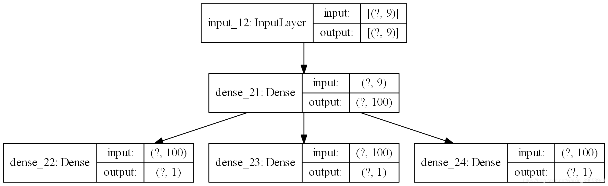
在训练模型时,每个样本需要三个独立的输出数组。我们可以通过将具有形状[7,3]的输出训练数据转换为具有形状[7,1]的三个数组来实现:
# separate output
y1 = y[:, 0].reshape((y.shape[0], 1))
y2 = y[:, 1].reshape((y.shape[0], 1))
y3 = y[:, 2].reshape((y.shape[0], 1))
训练模型:
model.fit(X, [y1,y2,y3], epochs=2000, verbose=0)
完整代码:
from tensorflow.keras.models import Model
from tensorflow.keras.layers import Input, Dense
from tensorflow.keras.utils import plot_model
import numpy as np

def split_sequences(sequence, sliding_window_width):
    X, y = [], []
    for i in range(len(sequence)):
        # 找到最后一次滑动所截取数据中最后一个元素的索引,
        # 如果这个索引超过原序列中元素的索引则不截取;
        end_element_index = i + sliding_window_width
        if end_element_index > len(sequence) - 1: # 序列中最后一个元素的索引
            break

        sequence_x, sequence_y = sequence[i:end_element_index, :], sequence[end_element_index, :] # 取最后一列元素作为预测值y
        X.append(sequence_x)
        y.append(sequence_y)

    #return X,y
    return np.array(X), np.array(y)

def multi_output_model(n_input, y, epochs_num):
    visible = Input(shape=(n_input,))
    dense = Dense(100, activation='relu')(visible)

    output1 = Dense(1)(dense)
    output2 = Dense(1)(dense)
    output3 = Dense(1)(dense)

    model = Model(inputs=visible, outputs=[output1, output2, output3])
    model.compile(optimizer='adam', loss='mse')

    plot_model(model, to_file='multi_output_model.png', show_shapes=True, show_layer_names=True, rankdir='TB', dpi=200)

    model.fit(X, y, epochs=2000, verbose=0)

    return model

if __name__ == '__main__':
    sw_width = 3
    epochs_num = 2000

    # 训练数据
    in_seq1 = np.array([10, 20, 30, 40, 50, 60, 70, 80, 90])
    in_seq2 = np.array([15, 25, 35, 45, 55, 65, 75, 85, 95])
    out_seq = np.array([in_seq1[i]+in_seq2[i] for i in range(len(in_seq1))])

    in_seq1 = in_seq1.reshape((len(in_seq1), 1))
    in_seq2 = in_seq2.reshape((len(in_seq2), 1))
    out_seq = out_seq.reshape((len(out_seq), 1))

    dataset = np.hstack((in_seq1, in_seq2, out_seq))

    # 训练数据和标签划分
    X, y = split_sequences(dataset, sw_width)

    print(X.shape, y.shape)
#     for i in range(len(X)):
#         print(X[i], y[i])

    n_input = X.shape[1] * X.shape[2]
    X = X.reshape((X.shape[0], n_input))

    y1 = y[:, 0].reshape((y.shape[0], 1))
    y2 = y[:, 1].reshape((y.shape[0], 1))
    y3 = y[:, 2].reshape((y.shape[0], 1))
    y_list = [y1,y2,y3]

    model = multi_output_model(n_input, y_list, epochs_num)

    x_input = np.array([[70,75,145], [80,85,165], [90,95,185]])
    x_input = x_input.reshape((1, n_input))
    yhat = model.predict(x_input, verbose=0)
    print(yhat)
输出:
(6, 3, 3) (6, 3)
[array([[100.50821]], dtype=float32), array([[105.74859]], dtype=float32), array([[206.86055]], dtype=float32)]
4. 多步MLP模型(Multi-step MLP Models)
实际上,MLP模型在预测表示不同输出变量的向量输出(如前一示例中所示)或表示一个变量的多个时间步的向量输出方面几乎没有差别。然而,在训练数据的准备方式上存在着微妙而重要的差异。
4.1 数据准备
与一步预测一样,用于多步时间序列预测的时间序列必须分成具有输入和输出分量的样本。输入和输出分量将由多个时间步组成,并且可能具有或可能不具有相同的步数。例如,给定一元时间序列:
[10, 20, 30, 40, 50, 60, 70, 80, 90]
我们可以使用三个时间步骤作为输入,并预测下两个时间步骤。第一个样本如下:
输入:
[10, 20, 30]
输出:
[40, 50]
数据划分结果:
[10 20 30] [40 50]
[20 30 40] [50 60]
[30 40 50] [60 70]
[40 50 60] [70 80]
[50 60 70] [80 90]
4.2 Vector Output Model
MLP可以直接输出一个可以解释为多步预测的向量。该方法在前一节中看到,每个输出时间序列的一个时间步长被预测为一个向量。在n步输入和n步输出变量中指定输入和输出步数,就可以定义一个多步时间序列预测模型。
完整代码:
from tensorflow.keras.models import Sequential
from tensorflow.keras.layers import Dense
import numpy as np

def split_sequence(sequence, m_steps_in, n_steps_out):
    X, y = [], []
    for i in range(len(sequence)):

        end_element_index = i + n_steps_in
        out_end_index = end_element_index + n_steps_out
        if out_end_index > len(sequence):
            break

        sequence_x, sequence_y = sequence[i:end_element_index], sequence[end_element_index:out_end_index]
        X.append(sequence_x)
        y.append(sequence_y)

    return np.array(X), np.array(y)

def vector_output_model(n_steps_in, n_steps_out, X, y, epochs_num):
    model = Sequential()
    model.add(Dense(100, activation='relu', input_dim=n_steps_in))
    model.add(Dense(n_steps_out))
    model.compile(optimizer='adam', loss='mse')

    model.fit(X, y, epochs=2000, verbose=0)
    return model

if __name__ == '__main__':
    epochs_num = 2000
    n_steps_in, n_steps_out = 3, 2

    raw_seq = [10, 20, 30, 40, 50, 60, 70, 80, 90]
    X, y = split_sequence(raw_seq, n_steps_in, n_steps_out)

    print(X.shape, y.shape)
    for i in range(len(X)):
        print(X[i], y[i])

    model = vector_output_model(n_steps_in, n_steps_out, X, y, epochs_num)

    x_input = np.array([70, 80, 90])
    x_input = x_input.reshape((1, n_steps_in))
    yhat = model.predict(x_input, verbose=0)
    print(yhat)
输出:
(5, 3) (5, 2)
[10 20 30] [40 50]
[20 30 40] [50 60]
[30 40 50] [60 70]
[40 50 60] [70 80]
[50 60 70] [80 90]
[[100.4229  111.65523]]
5 多元多步MLP模型(Multivariate Multi-step MLP Models)
在前面的章节中,我们讨论了单变量、多变量和多步时间序列预测。对于不同的问题,组合不同类型的MLP模型可能解决不同的问题。这也适用于涉及多变量和多步预测的时间序列预测问题,但这可能更具挑战性,特别是在准备数据和定义模型的输入和输出形状方面。
5.1 多输入多步输出
在多变量时间序列预测问题中,输出序列是独立的,但依赖于输入序列,输出序列需要多个时间步。例如,考虑前面一节中的多元时间序列:
[[ 10 15 25]
[ 20 25 45]
[ 30 35 65]
[ 40 45 85]
[ 50 55 105]
[ 60 65 125]
[ 70 75 145]
[ 80 85 165]
[ 90 95 185]]
我们可以使用两个输入时间序列中每一个的三个先验时间步来预测输出时间序列的两个时间步。
输入:
10, 15
20, 25
30, 35
输出:
65
85
完整代码:
from tensorflow.keras.models import Sequential
from tensorflow.keras.layers import Dense
import numpy as np

def split_sequences(sequences, n_steps_in, n_steps_out):
    X, y = [], []
    for i in range(len(sequences)):

        end_element_index = i + n_steps_in
        out_end_index = end_element_index + n_steps_out - 1

        if out_end_index > len(sequences):
            break

        sequence_x, sequence_y = sequences[i:end_element_index,:-1], sequences[end_element_index-1:out_end_index,-1]
        X.append(sequence_x)
        y.append(sequence_y)

    return np.array(X), np.array(y)

def multi_step_output_model(n_input, n_steps_out, X, y, epochs_num):
    model = Sequential()
    model.add(Dense(100, activation='relu', input_dim=n_input))
    model.add(Dense(n_steps_out))
    model.compile(optimizer='adam', loss='mse')

    model.fit(X, y, epochs=epochs_num, verbose=0)
    return model

if __name__ == '__main__':
    epochs_num = 2000

    in_seq1 = np.array([10, 20, 30, 40, 50, 60, 70, 80, 90])
    in_seq2 = np.array([15, 25, 35, 45, 55, 65, 75, 85, 95])
    out_seq = np.array([in_seq1[i]+in_seq2[i] for i in range(len(in_seq1))])

    in_seq1 = in_seq1.reshape((len(in_seq1), 1))
    in_seq2 = in_seq2.reshape((len(in_seq2), 1))
    out_seq = out_seq.reshape((len(out_seq), 1))

    dataset = np.hstack((in_seq1, in_seq2, out_seq))

    n_steps_in, n_steps_out = 3, 2

    X, y = split_sequences(dataset, n_steps_in, n_steps_out)

    n_input = X.shape[1] * X.shape[2]
    X = X.reshape((X.shape[0], n_input))

    print(X.shape, y.shape)
    for i in range(len(X)):
        print(X[i], y[i])

    model = multi_step_output_model(n_input, n_steps_out, X, y, epochs_num)

    x_input = np.array([[70, 75], [80, 85], [90, 95]])
    x_input = x_input.reshape((1, n_input))
    yhat = model.predict(x_input, verbose=0)
    print(yhat)
输出:
(6, 6) (6, 2)
[10 15 20 25 30 35] [65 85]
[20 25 30 35 40 45] [ 85 105]
[30 35 40 45 50 55] [105 125]
[40 45 50 55 60 65] [125 145]
[50 55 60 65 70 75] [145 165]
[60 65 70 75 80 85] [165 185]
[[186.31998 206.29776]]
5.2 多并行输入多步输出
具有并行时间序列的问题可能需要预测每个时间序列的多个时间步。例如,考虑前面一节中的多元时间序列:
[[ 10 15 25]
[ 20 25 45]
[ 30 35 65]
[ 40 45 85]
[ 50 55 105]
[ 60 65 125]
[ 70 75 145]
[ 80 85 165]
[ 90 95 185]]
我们可以使用三个时间序列中每个时间序列的三个时间步作为模型的输入,并预测三个时间序列中每个时间步的下一个时间步作为输出。训练数据集中的第一个示例如下:
输入:
10, 15, 25
20, 25, 45
30, 35, 65
输出:
40, 45, 85
50, 55, 105
我们可以看到数据集的输入(X)和输出(Y)元素对于样本数量、时间步长和变量或并行时间序列来说都是三维的。
我们现在可以开发一个多变量多步预测的MLP模型。除了像前面的例子中那样使输入数据的形状扁平化外,我们还必须使输出数据的三维结构扁平化。这是因为MLP模型只能接受向量输入和输出。
# flatten input
n_input = X.shape[1] * X.shape[2]
X = X.reshape((X.shape[0], n_input))
# flatten output
n_output = y.shape[1] * y.shape[2]
y = y.reshape((y.shape[0], n_output))
完整代码:
from tensorflow.keras.models import Sequential
from tensorflow.keras.layers import Dense
import numpy as np

def split_sequences(sequences, n_steps_in, n_steps_out):
    X, y = [], []
    for i in range(len(sequences)):

        end_element_index = i + n_steps_in
        out_end_index = end_element_index + n_steps_out

        if out_end_index > len(sequences):
            break

        sequence_x, sequence_y = sequences[i:end_element_index,:], sequences[end_element_index:out_end_index,:]
        X.append(sequence_x)
        y.append(sequence_y)

    return np.array(X), np.array(y)

def multi_parallel_output_model(n_input, n_output, X, y, epochs_num):
    model = Sequential()
    model.add(Dense(100, activation='relu', input_dim=n_input))
    model.add(Dense(n_output))
    model.compile(optimizer='adam', loss='mse')

    model.fit(X, y, epochs=epochs_num, verbose=0)
    return model

if __name__ == '__main__':
    epochs_num = 2000

    in_seq1 = np.array([10, 20, 30, 40, 50, 60, 70, 80, 90])
    in_seq2 = np.array([15, 25, 35, 45, 55, 65, 75, 85, 95])
    out_seq = np.array([in_seq1[i]+in_seq2[i] for i in range(len(in_seq1))])

    in_seq1 = in_seq1.reshape((len(in_seq1), 1))
    in_seq2 = in_seq2.reshape((len(in_seq2), 1))
    out_seq = out_seq.reshape((len(out_seq), 1))
    # 沿列堆叠数组,相当于列数增加
    dataset = np.hstack((in_seq1, in_seq2, out_seq))
    # 时间步长
    n_steps_in, n_steps_out = 3, 2
    # 将输入数据分为训练数据和训练标签
    X, y = split_sequences(dataset, n_steps_in, n_steps_out)
    # 展平输入数据
    n_input = X.shape[1] * X.shape[2]
    X = X.reshape((X.shape[0], n_input))
    # 展平输出数据
    n_output = y.shape[1] * y.shape[2]
    y = y.reshape((y.shape[0], n_output))

    print(X.shape, y.shape)
    for i in range(len(X)):
        print(X[i], y[i])

    model = multi_parallel_output_model(n_input, n_output, X, y, epochs_num)

    x_input = np.array([[60, 65, 125], [70, 75, 145], [80, 85, 165]])
    x_input = x_input.reshape((1, n_input))
    yhat = model.predict(x_input, verbose=0)
    print(yhat)
输出:
(5, 9) (5, 6)
[10 15 25 20 25 45 30 35 65] [ 40  45  85  50  55 105]
[20 25 45 30 35 65 40 45 85] [ 50  55 105  60  65 125]
[ 30  35  65  40  45  85  50  55 105] [ 60  65 125  70  75 145]
[ 40  45  85  50  55 105  60  65 125] [ 70  75 145  80  85 165]
[ 50  55 105  60  65 125  70  75 145] [ 80  85 165  90  95 185]
[[ 92.22672   96.749825 188.34888  102.91172  108.4422   209.61449 ]]
