普通线性回归
1.最小二乘线性模型
> dat=read.csv("https://raw.githubusercontent.com/happyrabbit/DataScientistR/master/Data/SegData.csv")
> dat=subset(dat,store_exp >0&online_exp >0)
> modeldat=dat[,grep("Q",names(dat))]
> modeldat$total_exp=dat$store_exp+dat$online_exp
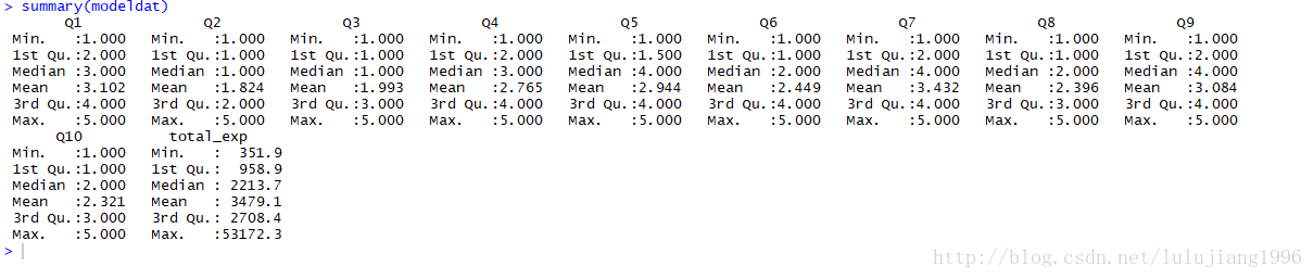
下面展示输出结果,看哈数据是否有缺失值或离群点
> par(mfrow=c(1,2))
> hist(modeldat$total_exp,main="",xlab="total_exp")
> boxplot(modeldat$total_exp)
> 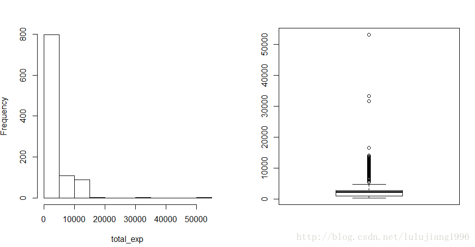
如上,数据集modeldat中没有缺失值,但是明显有离群点,而且因变量total_exp分布明显偏离正太。
我们需要删除离群点,然后对因变量进行对数变换
我们用Z分值的方法查找并删除离群点。
> y=modeldat$total_exp
 #求z分值
> zs=(y-mean(y))/mad(y)
 #找到z分值大于3.5的离群点,删除这些观测
> modeldat=modeldat[-which(zs>3.5),]
>
接下来检查变量的共线性
> library(corrplot)
corrplot 0.84 loaded
Warning message:
程辑包‘corrplot’是用R版本3.4.3 来建造的
> correlation=cor(modeldat[,grep("Q",names(modeldat))])
> corrplot.mixed(correlation,order="hclust",tl.pos="lt",upper="ellipse")
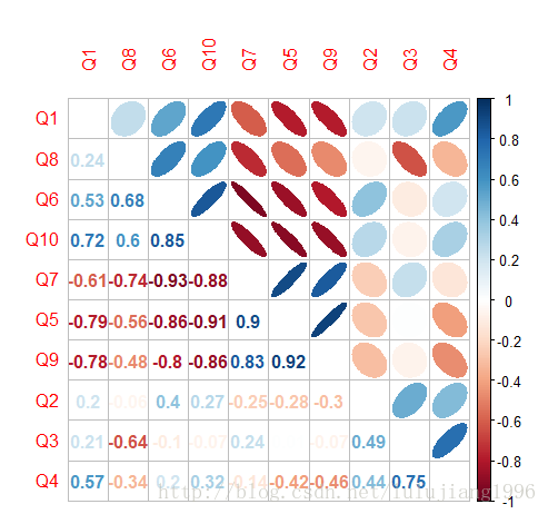
由上图可以看出,变量之间有很强的相关性。
我们需要删除高度相关变量的算法,设置阈值为0.75
> library(caret)
载入需要的程辑包:lattice
载入需要的程辑包:ggplot2
Warning messages:
1: 程辑包‘caret’是用R版本3.4.3 来建造的
2: 程辑包‘lattice’是用R版本3.4.3 来建造的
3: 程辑包‘ggplot2’是用R版本3.4.3 来建造的
> highcor=findCorrelation(correlation,cutoff=.75)
> modeldat=modeldat[,-highcor]
现在我们可以拟合线性模型。“.“表示数据集modeldat中除了因变量外所有的变量都被当做自变量,这里我们没有考虑交互效应。
且我们对原始变量进行了对数变换
> limfit=lm(log(total_exp)~.,data=modeldat)
> summary(lmfit)
Error in summary(lmfit) : object 'lmfit' not found
> summary(limfit)

Call:
lm(formula = log(total_exp) ~ ., data = modeldat)

Residuals:
     Min       1Q   Median       3Q      Max
-1.17494 -0.13719  0.01284  0.14163  0.56227

Coefficients:
             Estimate Std. Error t value Pr(>|t|)
(Intercept)  8.098314   0.054286 149.177  < 2e-16 ***
Q1          -0.145340   0.008823 -16.474  < 2e-16 ***
Q2           0.102275   0.019492   5.247 1.98e-07 ***
Q3           0.254450   0.018348  13.868  < 2e-16 ***
Q6          -0.227684   0.011520 -19.764  < 2e-16 ***
Q8          -0.090706   0.016497  -5.498 5.15e-08 ***
---
Signif. codes:  0 ‘***’ 0.001 ‘**’ 0.01 ‘*’ 0.05 ‘.’ 0.1 ‘ ’ 1

Residual standard error: 0.2262 on 805 degrees of freedom
Multiple R-squared:  0.8542,    Adjusted R-squared:  0.8533
F-statistic: 943.4 on 5 and 805 DF,  p-value: < 2.2e-16

>
我们也可以得到置信区间
> confint(limfit,level=0.9)
                    5 %        95 %
(Intercept)  8.00891811  8.18771037
Q1          -0.15986889 -0.13081186
Q2           0.07017625  0.13437445
Q3           0.22423576  0.28466333
Q6          -0.24665434 -0.20871330
Q8          -0.11787330 -0.06353905
>
2.回归诊断
根据高斯-马尔科夫定理,OLS(最小二乘估计)在下面条件满足时是BLUE(最优线性无偏估计):
(1)自变量和随机误差不相关
(2) 随机误差均值为0
(3)随机误差方差一致且相互独立
4种图形诊断
a.残差图(Residuals vs Fittled)
我们要检查残差图如下几个方面:
(1)残差是否分布在0附件
(2)残差分布是否随机,如果呈现出某种特定分布模式的话(如,随着横坐标的增大而增大或减小),说明当前模型关系的假设不充分。
(3)残差是否存在异方差性,比如随着拟合值增大残差分布方差增加,这就说明残差分布有异方差性。
当存在异方差时,参数估计值虽然是无偏的,但不是最小方差线性无偏估计。
由于参数的显著性检验是基于残差分布假设的,所以在该假设不成立的情况下该检验也将失效。如果你用该回归方程来预测新样本,效果可能不理想。
b.q-q图(Norm Q-Q)
它是一种正太分布检验。
对于标准正太分布,qq图上的点分布在y=x直线上,点偏离直线越远说明样本偏离正太分布越远。
c.标准化残差方根散点图(Scale-Location)
和残差图类似,横坐标依旧是样本拟合值,纵坐标为标准化残差的绝对值开方
d.Cook距离图(Cook’s distance)
该图用于判断观测值是否有异常点。
一般情况下,当D<0.5时认为不是异常值点;当D>0.5时认为是异常值点。
> par(mfrow=c(2,2))
> plot(lmfit,which=1)
Error in plot(lmfit, which = 1) : object 'lmfit' not found
> plot(limfit,which=1)
> plot(limfit,which=2)
> plot(limfit,which=3)
> plot(limfit,which=4)
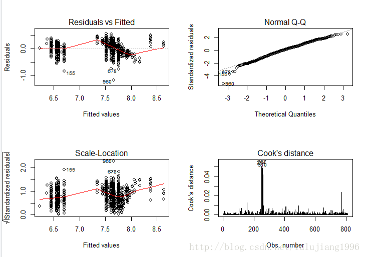
如上图
残差图:数据点都基本均匀分布在直线y=0两侧,无明显趋势,满足线性假设。
标准Q-Q图:图上的点基本度在y=x直线附件,可认为残差近似服从正太分布
标准化残差方根散点图:若满足不变方差假设,则在该图中水平线周围的点应该随机分布,最高点为残差最大值点。该图显示基本符合方差齐性的要求。
Cook距离图:最大的Cook距离为0.05左右,可以认为没有异常点。
3.离群点,高杠杆点和强影响点
离群点:
Cook距离图,Z分值都可以用来检验线性模型中的离群点。
但是,Z分值仅仅是针对因变量观测而言,和使用模型无关,其并未考虑模型的拟合情况。
car包中的outlierTest()函数可以用于对拟合模型对象检验是否存在离群点。
注意:这里的离群点指的是那些模型预测效果不佳的观测点。通常有很大的或正或负的残差,正残差说明模型低估了响应值,负残差说明高估了响应值。这里使用的是Bonferroni离群点检验,该检验也可作用于广义线性模型。
对于一般线性模型使用的是t检验,对于广义线性模型使用的是正太检验。
> library(car)
Warning message:
程辑包‘car’是用R版本3.4.3 来建造的
> outlierTest(limfit)
     rstudent unadjusted p-value Bonferonni p
960 -5.295504          1.533e-07   0.00012432
>
outlierTest()函数根据单个最大(正或负)残差值的显著性来判断是否有离群点,若不显著,则说明数据集中没有离群点,若显著,则检验删除该离群点,然后再检验是否还有其他离群点存在。
如上,这里需要删除第960个被认为是离群点的观测。
> outlierTest(limfit)
     rstudent unadjusted p-value Bonferonni p
960 -5.295504          1.533e-07   0.00012432
#找到相应的观测
> idex=which(row.names(modeldat)=="960")
#删除离群观测
> modeldat=modeldat[-idex,]
>
接下来我们再拟合一次模型,然后检验看看是否还有离群点。
> limfit=lm(log(total_exp)~.,data=modeldat)
> outlierTest(limfit)

No Studentized residuals with Bonferonni p < 0.05
Largest |rstudent|:
     rstudent unadjusted p-value Bonferonni p
155 -3.818112         0.00014483      0.11731
>
如上,可以看出,现在没有检验出显著离群点。
高杠杆值点:
高杠杆值点是与其他预测变量又关的离群点,即它们是由许多异常的预测变量组合起来的,与响应变量值没有关系。
高杠杆值的观测点可通过帽子矩阵的值(hat statistic)来判断。
对于一个给定的数据集,帽子均值为p/n,p是模型估计的参数数目(包含截距项),n是样本量。
一般来说,若观测点的帽子值大于帽子均值的2或3倍,则可认定为高杠杆值点。
收缩方法
收缩方法属于内嵌法。
我们可以对模型参数进行限制或者规范化来达到变量选择的效果,这些方法能将一些参数估计朝着0收缩。
1.岭回归
R中可以进行岭回归的函数
MASS包中的Im.ridge()函数
elasticnet包中的enet()函数
若需要对参数进行优化,最方便的是caret包中的train函数
> dat=read.csv("https://raw.githubusercontent.com/happyrabbit/DataScientistR/master/Data/SegData.csv")
> dat=subset(dat,store_exp>0&online_exp>0)
> trainx=dat[,grep("Q",names(dat))]
> trainy=dat$store_exp+dat$online_exp
先用train函数对参数进行调优
首先设置交互校验和参数调优范围,这里我们使用10层交互校验。
为了保险起见,在用此类方法前应进行标准化
> ctr1=trainControl(method="cv",number=10)
> ridgeGrid=data.frame(.lambda=seq(0,.1,length=20))
> set.seed(100)
> ridgeRegTune=train(trainx,trainy,method="ridge",

#用不同罚函数值来拟合模型
tuneGrid=ridgeGrid,trControl=ctr1,
#中心化和标度化变量
preProc=c("center","scale"))
> ridgeRegTune
Ridge Regression

999 samples
 10 predictor

Pre-processing: centered (10), scaled (10)
Resampling: Cross-Validated (10 fold)
Summary of sample sizes: 899, 899, 899, 899, 899, 899, ...
Resampling results across tuning parameters:

  lambda       RMSE      Rsquared   MAE
  0.000000000  1748.466  0.7942143  752.9785
  0.005263158  1748.281  0.7943720  753.6987
  0.010526316  1748.549  0.7944728  754.6125
  0.015789474  1749.154  0.7945374  755.7452
  0.021052632  1750.026  0.7945778  757.0960
  0.026315789  1751.121  0.7946015  758.6035
  0.031578947  1752.411  0.7946132  760.2972
  0.036842105  1753.875  0.7946162  762.1418
  0.042105263  1755.500  0.7946125  764.1251
  0.047368421  1757.276  0.7946037  766.1779
  0.052631579  1759.193  0.7945909  768.2752
  0.057894737  1761.246  0.7945750  770.5444
  0.063157895  1763.430  0.7945564  772.9384
  0.068421053  1765.739  0.7945357  775.3503
  0.073684211  1768.171  0.7945131  777.9338
  0.078947368  1770.721  0.7944890  780.5918
  0.084210526  1773.387  0.7944636  783.3492
  0.089473684  1776.166  0.7944370  786.1977
  0.094736842  1779.055  0.7944094  789.2161
  0.100000000  1782.051  0.7943808  792.3606

RMSE was used to select the optimal model using the smallest value.
The final value used for the model was lambda = 0.005263158.
>
如上,训练出的模型调优参数为0.01,对应RMSE和R^2分别为1748.281和80%
下面展示如何使用elasticnet包中的enet()函数
> library(elasticnet)
载入需要的程辑包:lars
Loaded lars 1.2

> ridgefit=enet(x=as.matrix(trainx),y=trainy,lambda=0.01,
 #设置将自变量标准化
 normalize=TRUE)
> ridgePred=predict(ridgefit,newx=as.matrix(trainx),s=1,mode="fraction",type="fit")
> names(ridgePred)
[1] "s"        "fraction" "mode"     "fit"
> head(ridgePred$fit)
        1         2         3         4         5         6
1290.4697  224.1595  591.4406 1220.6384  853.3572  908.2040
要得到参数拟合结果,需要在predict()函数中设定type=”coefficients”
> ridgeCoef=predict(ridgefit,newx=as.matrix(trainx),s=1,mode="fraction",type="coefficients")
> RidgeCoef=ridgeCoef$coefficients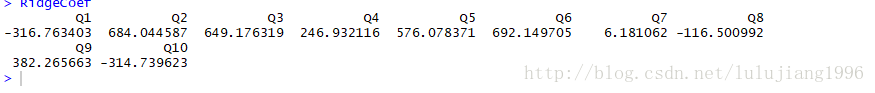
岭回归于原始最小二乘回归相比优势在于偏差和方差之间的权衡。
一般线性回归中的最小二乘估计在无偏估计中是最优的,但通常估计方差会很大,这意味着训练集数据的微小变化可能导致参数估计较大的变化。
岭回归估计就是通过牺牲一点点“无偏性”,换取估计方差的减少。
它更适合在普通最小二乘回归参数估计方差很大的情况下使用。
2.Lasso(具体过程等会在新篇里讲解)
虽然岭回归可以将参数估计值向0进行收缩,但对于任何调优参数值,它都不能将系数取值变为严格的0.
尽管某些参数估计值变得非常小以至于可以忽略,但事实上岭回归并没有进行变量选择。这可能对预测精确度来说不是问题,但对模型解释提出了挑战。
Lasso(最小绝对收缩与选择算子模型)出现用来代替岭回归模型。
Lasso和岭回归很相似,唯一不同的在于罚函数。
下面展示在R中如何进行调优和拟合
先用train()函数对参数进行调优
首先设置交互校验和参数调优范围,这里使用10层交互校检,在用该方法前注意要进行标准化
> ctr1=trainControl(method="cv",number=10)
> lassoGrid=data.frame(fraction=seq(.8,1,length=20))
> set.seed(100)
> lassoTune=train(trainx,trainy,method="lars",tuneGrid=lassoGrid,trControl=ctr1,preProc=c("center","scale"))
> lassoTune
Least Angle Regression

999 samples
 10 predictor

Pre-processing: centered (10), scaled (10)
Resampling: Cross-Validated (10 fold)
Summary of sample sizes: 899, 899, 899, 899, 899, 900, ...
Resampling results across tuning parameters:

  fraction   RMSE      Rsquared   MAE
  0.8000000  1762.679  0.7921007  787.5439
  0.8105263  1760.384  0.7924426  784.0889
  0.8210526  1758.364  0.7927419  780.8319
  0.8315789  1756.401  0.7930346  777.7173
  0.8421053  1754.409  0.7933317  774.6333
  0.8526316  1752.524  0.7936236  771.8127
  0.8631579  1750.750  0.7939136  769.0883
  0.8736842  1749.101  0.7941909  766.5841
  0.8842105  1747.581  0.7944455  764.3044
  0.8947368  1746.207  0.7946761  762.1525
  0.9052632  1745.021  0.7948805  760.1038
  0.9157895  1744.029  0.7950563  758.3066
  0.9263158  1743.229  0.7952038  756.7197
  0.9368421  1742.674  0.7953067  755.4797
  0.9473684  1742.382  0.7953591  754.5233
  0.9578947  1742.284  0.7953832  753.9641
  0.9684211  1742.380  0.7953767  753.5812
  0.9789474  1742.667  0.7953442  753.4000
  0.9894737  1743.178  0.7952871  753.5050
  1.0000000  1743.953  0.7951834  754.0392

RMSE was used to select the optimal model using the smallest value.
The final value used for the model was fraction = 0.9578947.
>
训练出的模型调优参数为0.95,对应的RMSE和R^2分别为1742.284何80%,和之前的岭回归几乎相同。
> plot(lassoTune)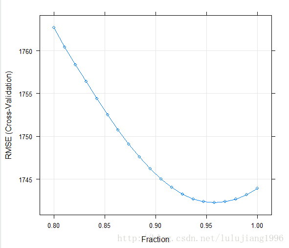
从上交互校验的RMSE结果图中可以看出,随着调优参数的增加,RMSE有一个减少然后增加的过程
Lasso模型可以用许多不同的函数进行拟合
lars包中的lars()函数
elasticnet包的enet()函数
glmnet包中的glmnet()函数
下面我们使用enet()函数,其要求自变量为一个矩阵对象,要讲数据框trainx转换成矩阵。
预测变量在建模之前需要中心化和标准化,函数中的normalize参数可以自动完成这一过程。
lambda参数控制了岭回归的罚参数
> lassoModel=enet(x=as.matrix(trainx),y=trainy,lambda=0,normalize=TRUE)
> lassoFit=predict(lassoModel,newx=as.matrix(trainx),s=.95,mode="fraction",type="fit")
> head(lassoFit$fit)
        1         2         3         4         5         6
1371.6160  308.6984  702.2026 1225.5508  832.0466 1028.9785
在predict()函数中设定type=”coefficients”
可以得到参数拟合结果
> lassoCoef=predict(lassoModel,newx=as.matrix(trainx),s=0.95,mode="fraction",type="coefficients")
> LassoCoef=lassoCoef$coefficients
> LassoCoef
       Q1        Q2        Q3        Q4        Q5        Q6        Q7        Q8        Q9       Q10
-326.7759  720.2801  722.7518  180.7107  542.1603  603.0865    0.0000  -75.9610  342.6375 -281.7818
3.弹性网络
它是Lasso的一般化版本,该模型结合了两种罚函数
Lasso对应的估计方差较大,而岭回归又没有特征选择的功能,弹性网络的优点在于利用了岭回归的罚函数,同时又由Lasso的特征选择功能。
该模型能够更有效地处理成组的高度相关变量。
> enetGrid=expand.grid(.lambda=seq(0,0.2,length=20),.fraction=seq(.8,1,length=20))
> set.seed(100)
> enetTune=train(trainx,trainy,method="enet",tuneGrid=enetGrid,trControl=ctrl,preProc=c("center","scale"))
Error in train.default(trainx, trainy, method = "enet", tuneGrid = enetGrid,  :
  object 'ctrl' not found
> enetTune=train(trainx,trainy,method="enet",tuneGrid=enetGrid,trControl=ctr1,preProc=c("center","scale"))
> enetfit=enet(x=as.matrix(trainx),y=trainy,lambda=0.01,normalize=TRUE)
> enetPred=predict(enetfit,newx=as.matrix(trainx),s=0.958,mode="fraction",type="fit")
> enetCoef=predict(ridgefit,newx=as.matrix(trainx),s=0.958,mode="fraction",type="coefficients")
> enetCoef
$s
[1] 0.958

$fraction
    0
0.958

$mode
[1] "fraction"

$coefficients
        Q1         Q2         Q3         Q4         Q5         Q6         Q7         Q8         Q9        Q10
-354.24218  744.20631  703.81744  189.47130  499.01455  586.62172    0.00000  -96.71702  352.72551 -284.57245

>
主成分和偏最小二乘回归
在实际应用中,自变量之间通常是彼此相关的,包含相似的信息。
如果对预测变量进行主成分分析(PCA),然后用主成分进行回归,这种方法得到的主成分是彼此不相关的。
但存在弊端是得到的新自变量是原变量的线性组合,因此使得模型难以理解。
偏最小二乘回归(PLS)是PCR的有监督版本
在建模前也需要进行标准化。(具体原理会在后面章节中专门讲解)
下面展示如何用R中的caret包训练PCR和PLS模型
> library(lattice)
> library(caret)
> library(dplyr)

载入程辑包:‘dplyr’

The following object is masked from ‘package:car’:

    recode

The following objects are masked from ‘package:stats’:

    filter, lag

The following objects are masked from ‘package:base’:

    intersect, setdiff, setequal, union

Warning message:
程辑包‘dplyr’是用R版本3.4.3 来建造的
> library(elasticnet)
> library(lars)
> sim.dat=read.csv("https://raw.githubusercontent.com/happyrabbit/DataScientistR/master/Data/SegData.csv")
> ymad=mad(na.omit(sim.dat$income))
> zs=(sim.dat$income-mean(na.omit(sim.dat$income)))/ymad
> idex=c(which(na.omit(zs>3.5)),which(is.na(zs)))
> sim.dat=sim.dat[-idex,]
> xtrain=dplyr::select(sim.dat,Q1:Q10)
> ytrain=sim.dat$income
> set.seed(100)
> ctr1=trainControl(method="cv",number=10)
> plsTune=train(xtrain,ytrain,method="pls",tuneGrid=expand.grid(.ncomp=1:10))
> plsTune=train(xtrain,ytrain,method="pls",tuneGrid=expand.grid(.ncomp=1:10),trControl=ctr1)
> plsTune
Partial Least Squares

772 samples
 10 predictor

No pre-processing
Resampling: Cross-Validated (10 fold)
Summary of sample sizes: 694, 696, 696, 696, 694, 695, ...
Resampling results across tuning parameters:

  ncomp  RMSE      Rsquared   MAE
   1     28106.40  0.6553646  19957.91
   2     24852.89  0.7385908  16142.37
   3     23594.19  0.7679501  14507.19
   4     23442.31  0.7713064  13940.47
   5     23407.49  0.7721321  13848.48
   6     23409.49  0.7720994  13838.38
   7     23408.15  0.7721470  13835.54
   8     23408.56  0.7721433  13835.52
   9     23408.46  0.7721447  13835.46
  10     23408.46  0.7721448  13835.48

RMSE was used to select the optimal model using the smallest value.
The final value used for the model was ncomp = 5.
>
如上,可以看到,调优的结果是选取7个主成分。
但其实在成分数目5之后RMSE变化就不太大了
从PLS调优过程中还可以得到变量的重要性排序。
今天就先到这里咯,明天继续~