基于XGBOOST的电能消耗预测

数据来源 ：Hourly Energy Consumption
PJM INT.，L.L.C.(以下简称为PJM)是经美国联邦能源管制委员会(FERC)批准，于1997的3月31日成立的一个非股份制有限责任公司，它实际上是一个独立系统运营商(ISO)。PJM目前负责美国13个州以及哥伦比亚特区电力系统的运行与管理。作为区域性ISO，PJM负责集中调度美国目前最大、最复杂的电力控制区，其规模在世界上处于第三位。PJM控制区人口占全美总人口的8.7%（约2300万人），负荷占7.5%，装机容量占8%(约58698MW)，输电线路长达12800多公里。

PJM拥有9个PJM输电网络所有者成员（Baltimore天然气&电力公司、Delmarva电类公司、Jersey中心电灯公司、Metropolitan爱迪生公司、PECO能源公司、宾夕法尼亚电力公司、PPL电力公用公司、Poromac电力公司、UGI公用有限公司）。

import numpy as np # linear algebra
import pandas as pd # data processing, CSV file I/O (e.g. pd.read_csv)
import seaborn as sns
import matplotlib.pyplot as plt
import xgboost as xgb
from xgboost import plot_importance, plot_tree
from sklearn.metrics import mean_squared_error, mean_absolute_error
plt.style.use('fivethirtyeight')

数据探索分析（EDA）

数据读取

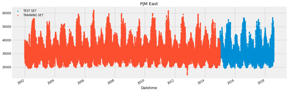
读取"PJM East" 的数据，包括了2002-2018 整个东部地区的用电数据。数据是以小时作为索引的。

pjme = pd.read_csv('input/PJME_hourly.csv', index_col=[0], parse_dates=[0])
pjme.head()

	PJME_MW
Datetime
2002-12-31 01:00:00	26498.0
2002-12-31 02:00:00	25147.0
2002-12-31 03:00:00	24574.0
2002-12-31 04:00:00	24393.0
2002-12-31 05:00:00	24860.0

数据可视化

color_pal = ["#F8766D", "#D39200", "#93AA00", "#00BA38", "#00C19F", "#00B9E3", "#619CFF", "#DB72FB"]
_ = pjme.plot(style='.', figsize=(15,5), color=color_pal[0], title='PJM East')

评价指标（metric）

这是一个回归任务，常用的评价指标为RMSE或者MAE，但是这两者衡量的是偏差（error）的绝对值，为了衡量偏差的相对值，还有一个指标MAPE。这三者的定义和关系如下。

这个任务中，这三个指标都可以用来衡量模型的性能。

训练集测试集（train_test_split）

将2015年之后的数据作为测试集

split_date = '01-Jan-2015'
pjme_train = pjme.loc[pjme.index <= split_date].copy()
pjme_test = pjme.loc[pjme.index > split_date].copy()
_ = pjme_test \
    .rename(columns={'PJME_MW': 'TEST SET'}) \
    .join(pjme_train.rename(columns={'PJME_MW': 'TRAINING SET'}), how='outer') \
    .plot(figsize=(15,5), title='PJM East', style='.')

基线模型（baseline）

最简单的做法就是直接用训练集的数据作为对测试集的预测，可以作为基线模型。

建立时序特征（time series）

pjme_train.iloc[0].index

Index(['PJME_MW'], dtype='object')

def create_features(df, label=None):
    """
    Creates atime series features from datetime index
    """
    df['date'] = df.index
    df['hour'] = df['date'].dt.hour
    df['dayofweek'] = df['date'].dt.dayofweek
    df['quarter'] = df['date'].dt.quarter
    df['month'] = df['date'].dt.month
    df['year'] = df['date'].dt.year
    df['dayofyear'] = df['date'].dt.dayofyear
    df['dayofmonth'] = df['date'].dt.day
    df['weekofyear'] = df['date'].dt.weekofyear
    
    X = df[['hour','dayofweek','quarter','month','year',
           'dayofyear','dayofmonth','weekofyear']]
    if label:
        y = df[label]
        return X, y
    return X

X_train, y_train = create_features(pjme_train, label='PJME_MW')
X_test, y_test = create_features(pjme_test, label='PJME_MW')

X_test.head()

	hour	dayofweek	quarter	month	year	dayofyear	dayofmonth	weekofyear
Datetime
2015-12-31 01:00:00	1	3	4	12	2015	365	31	53
2015-12-31 02:00:00	2	3	4	12	2015	365	31	53
2015-12-31 03:00:00	3	3	4	12	2015	365	31	53
2015-12-31 04:00:00	4	3	4	12	2015	365	31	53
2015-12-31 05:00:00	5	3	4	12	2015	365	31	53

数据建模

XGBoost 模型

reg = xgb.XGBRegressor(n_estimators=1000)
reg.fit(X_train, y_train,
        eval_set=[(X_train, y_train), (X_test, y_test)],
        early_stopping_rounds=50,
       verbose=False) # Change verbose to True if you want to see it train

D:\Anaconda3\lib\site-packages\xgboost\core.py:587: FutureWarning: Series.base is deprecated and will be removed in a future version
  if getattr(data, 'base', None) is not None and \
D:\Anaconda3\lib\site-packages\xgboost\core.py:588: FutureWarning: Series.base is deprecated and will be removed in a future version
  data.base is not None and isinstance(data, np.ndarray) \





XGBRegressor(base_score=0.5, booster='gbtree', colsample_bylevel=1,
             colsample_bytree=1, gamma=0, importance_type='gain',
             learning_rate=0.1, max_delta_step=0, max_depth=3,
             min_child_weight=1, missing=None, n_estimators=1000, n_jobs=1,
             nthread=None, objective='reg:linear', random_state=0, reg_alpha=0,
             reg_lambda=1, scale_pos_weight=1, seed=None, silent=True,
             subsample=1)

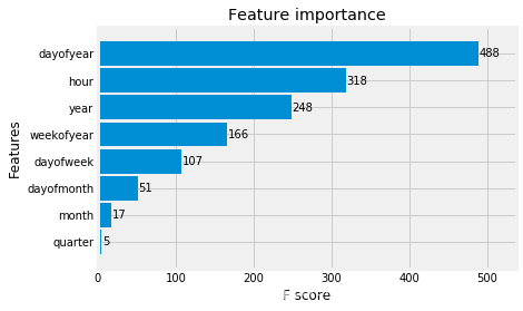
特征重要性

sklearn 在训练后会自动计算每个特征的重要度。我们可以通过 feature_importances_ 变量来查看结果。我们可以观察到，day of year是最重要的特征，然后才是hour和year。quarter的重要性很低。

_ = plot_importance(reg, height=0.9)

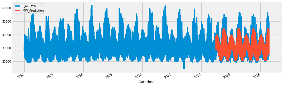
测试集预测

pjme_test['MW_Prediction'] = reg.predict(X_test)
pjme_all = pd.concat([pjme_test, pjme_train], sort=False)

_ = pjme_all[['PJME_MW','MW_Prediction']].plot(figsize=(15, 5))

结果分析

测试集的评测指标

对于回归任务，有三个常用评测指标，RMSE，MAE和MAPE。MAPE能够很好的衡量误差的百分比，但是在sklearn中没有提供，需要自己定义。对于这个数据集，我们得到这三个指标分别为

指标（metric）	结果（result）
RMSE	13780445
MAE	2848.89
MAPE	8.9%

mean_squared_error(y_true=pjme_test['PJME_MW'],
                   y_pred=pjme_test['MW_Prediction'])

13780445.55710396

mean_absolute_error(y_true=pjme_test['PJME_MW'],
                   y_pred=pjme_test['MW_Prediction'])

2848.891429322955

def mean_absolute_percentage_error(y_true, y_pred): 
    """Calculates MAPE given y_true and y_pred"""
    y_true, y_pred = np.array(y_true), np.array(y_pred)
    return np.mean(np.abs((y_true - y_pred) / y_true)) * 100

mean_absolute_percentage_error(y_true=pjme_test['PJME_MW'],
                   y_pred=pjme_test['MW_Prediction'])

8.94944673745318

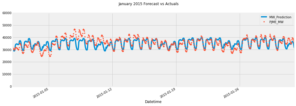
第一个月的预测结果

# Plot the forecast with the actuals
f, ax = plt.subplots(1)
f.set_figheight(5)
f.set_figwidth(15)
_ = pjme_all[['MW_Prediction','PJME_MW']].plot(ax=ax,
                                              style=['-','.'])
ax.set_xbound(lower='01-01-2015', upper='02-01-2015')
ax.set_ylim(0, 60000)
plot = plt.suptitle('January 2015 Forecast vs Actuals')

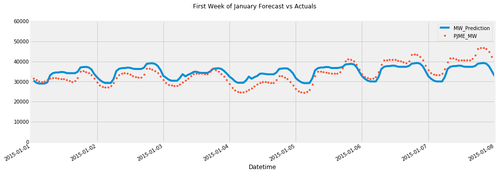
# Plot the forecast with the actuals
f, ax = plt.subplots(1)
f.set_figheight(5)
f.set_figwidth(15)
_ = pjme_all[['MW_Prediction','PJME_MW']].plot(ax=ax,
                                              style=['-','.'])
ax.set_xbound(lower='01-01-2015', upper='01-08-2015')
ax.set_ylim(0, 60000)
plot = plt.suptitle('First Week of January Forecast vs Actuals')

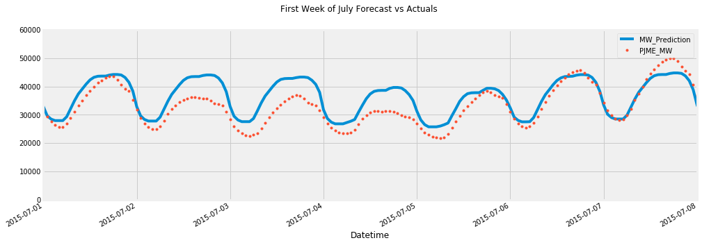
f, ax = plt.subplots(1)
f.set_figheight(5)
f.set_figwidth(15)
_ = pjme_all[['MW_Prediction','PJME_MW']].plot(ax=ax,
                                              style=['-','.'])
ax.set_ylim(0, 60000)
ax.set_xbound(lower='07-01-2015', upper='07-08-2015')
plot = plt.suptitle('First Week of July Forecast vs Actuals')

根据error降序排序

对测试集的预测结果增加两列，分别是‘error’，‘abs_error’。然后对abs_error按照天来求平均，得到每天的MAE。然后按照error排序。

节假日的预测结果都偏小。如果增加一个节假日的特征，应该对预测的结果有好处。

• 7月4日 - 美国国庆.
• 12月25日 - 圣诞节

pjme_test['error'] = pjme_test['PJME_MW'] - pjme_test['MW_Prediction']
pjme_test['abs_error'] = pjme_test['error'].apply(np.abs)
error_by_day = pjme_test.groupby(['year','month','dayofmonth']) \
    .mean()[['PJME_MW','MW_Prediction','error','abs_error']]

# Over forecasted days
error_by_day.sort_values('error', ascending=True).head(10)

			PJME_MW	MW_Prediction	error	abs_error
year	month	dayofmonth
2016	7	4	28399.958333	36986.964844	-8587.006429	8587.006429
2017	2	24	26445.083333	33814.503906	-7369.422445	7369.422445
2015	12	25	24466.083333	31584.923828	-7118.841390	7118.841390
2017	2	20	27070.583333	34100.781250	-7030.197754	7030.197754
2015	7	3	30024.875000	37021.031250	-6996.156169	6996.156169
2017	6	28	30531.208333	37526.589844	-6995.380371	6995.380371
	2	8	28523.833333	35511.699219	-6987.864258	6987.864258
	9	2	24201.458333	31180.390625	-6978.933105	6978.933105
	2	25	24344.458333	31284.279297	-6939.820150	6939.820150
2018	2	21	27572.500000	34477.417969	-6904.919352	6904.919352

按照abs_error 降序排序

那些预测的最好的天，似乎总是在十月份，因为十月份没有太多的节假日，气候也较为温和。

# Worst absolute predicted days
error_by_day.sort_values('abs_error', ascending=False).head(10)

			PJME_MW	MW_Prediction	error	abs_error
year	month	dayofmonth
2016	8	13	45185.833333	31753.224609	13432.608887	13432.608887
		14	44427.333333	31058.818359	13368.514404	13368.514404
	9	10	40996.166667	29786.179688	11209.987793	11209.987793
		9	43836.958333	32831.035156	11005.923828	11005.923828
2015	2	20	44694.041667	33814.503906	10879.535889	10879.535889
2018	1	6	43565.750000	33435.265625	10130.485921	10130.485921
2016	8	12	45724.708333	35609.312500	10115.394287	10115.394287
2017	5	19	38032.583333	28108.976562	9923.606689	9923.606689
	12	31	39016.000000	29314.683594	9701.315430	9701.315430
2015	2	21	40918.666667	31284.279297	9634.388184	9634.388184

按照abs_error 升序排序

# Best predicted days
error_by_day.sort_values('abs_error', ascending=True).head(10)

			PJME_MW	MW_Prediction	error	abs_error
year	month	dayofmonth
2016	10	3	27705.583333	27775.351562	-69.768148	229.585205
2015	10	28	28500.958333	28160.875000	340.083740	388.023356
2016	10	8	25183.333333	25535.669922	-352.337402	401.017090
	5	1	24503.625000	24795.419922	-291.794515	428.289307
2017	10	29	24605.666667	24776.271484	-170.605225	474.628988
2016	9	16	29258.500000	29397.271484	-138.770833	491.070312
	3	20	27989.416667	27620.132812	369.284831	499.750488
	10	2	24659.083333	25134.919922	-475.836670	516.188232
2017	10	14	24949.583333	25399.728516	-450.145996	520.855794
2015	5	6	28948.666667	28710.271484	238.396077	546.640544

最好和最差的那一天

f, ax = plt.subplots(1)
f.set_figheight(5)
f.set_figwidth(10)
_ = pjme_all[['MW_Prediction','PJME_MW']].plot(ax=ax,
                                              style=['-','.'])
ax.set_ylim(0, 60000)
ax.set_xbound(lower='08-13-2016', upper='08-14-2016')
plot = plt.suptitle('Aug 13, 2016 - Worst Predicted Day')

f, ax = plt.subplots(1)
f.set_figheight(5)
f.set_figwidth(10)
_ = pjme_all[['MW_Prediction','PJME_MW']].plot(ax=ax,
                                              style=['-','.'])
ax.set_ylim(0, 60000)
ax.set_xbound(lower='10-03-2016', upper='10-04-2016')
plot = plt.suptitle('Oct 3, 2016 - Best Predicted Day')