Distributed representation, Hyperbolic Space, Gaussian/Graph Embedding 详细介绍

往期文章链接目录

Overview of various word representation and Embedding methods

Local Representation v.s. Distributed Representation

• One-hot encoding is local representation and is good for local generalization; distributed representation is good for global generalization.

Comparison between local generalization and global generalization:

Here is an example for better understanding this pair of concepts. Suppose now you have a bunch of ingredients and you’re able to cook 100 different meals with these ingredients.

• Local Representation way of cooking:

  • You cook every meal directly from these ingredients.
  • Suppose you cook several meals a lot, then you would be good at cooking these meals. If you want to cook something new but similar to these meals (concept of “local”), you would probably also cook them well. Here we say you have a good local generalization.

• Global Representation way of cooking:

  • You first cook some semi-finished products. from these ingredients and then cook every meal from these semi-finished products.
  • For every meal, you use all of semi-finished products. That means if you want your meal to be delicious, you have to improve the quality of these semi-finished products. Therefore, if one meal become more delicious, then all semi-finished products become better in general, which in turn make other meal more delicious (concept of “parameter sharing”). Here we say you have a good global generalization.

What are advantages of Distributed Representation over Local Representation?

• Representational power: distributed representation forms a more efficient code than localist representations. A localist representation using $n$ neurons can represent just $n$ different entities. A distributed representation using $n$ binary neurons can represent up to $2^n$ different entities.

• Continuity (in the mathematical sense): representing concepts in continuous vector spaces allows powerful gradient-based learning techniques such as back-propagation to be applied to many problems.

• Soft capacity limits: distributed representations typically have soft limits on how many concepts can be represented simultaneously.

Context-free word representation v.s. Contextual word representation

• Context-free word representation: a single word representation is generated for each word in the vocabulary.

  • Example: CBOW, Skip-gram, GloVe, MF (matrix factorization).

• Contextual word representation: the word representation depends on the context where that word occurs, meaning that the same word in different contexts can have different representations.

  • Example: ELMo, Bert, XLNet, ALBert, GPT (Generative Pre-Training).

From Euclidean space to non-Euclidean space

Geometry is a familiar field for the machine learning community; geometric ideas play an important role in many parts of machine learning. For example, we often study the convexity of functions, the dimensionality and projections of data representations, and we frequently produce visualizations to understand our data and training processes.

In machine laerning, most of the times, we’ve actually imposed a geometry. We’ve chosen to work with Euclidean space, with all of its inherent properties, among the most critical of which is its flatness. However, the Euclidean space cannot handle all the cases and we still need to work with other spaces to solve some problems. Below, I list two advantages of non-Euclidean space:

• Better representations: Euclidean space simply doesn’t fit many types of data structures that we often need to work with. The core example is the hierarchy, or, its abstract network representation, the tree. There is a specific non-Euclidean choice that naturally fits trees: hyperbolic space, and I’m going to talk a little bit about it later.

• More flexible operations: The flatness of Euclidean space means that certain operations require a large number of dimensions and complexity to perform—while non-Euclidean spaces can potentially perform these operations in a more flexible way, with fewer dimensions.

Hyperbolic Space

A specific and common non-Euclidean space is the hyperbolic space, which is a good fit for the hierarchical representation. Here I am going to show two examples.

Example 1:

Suppose we want a model to learn the embeddings for the following four words: “Country”, “Asia”, “China”, and “Japan”. Apparently, there is a tree structure between these words. “Country” is the root node; “Asia” is a child node of “Country”; “China” and “Japan” are two sibling nodes and also child nodes of “Asia”. Therefore, we want our learned embeddings, in some degree, show this hierarchical structure. The Euclidean space cannot achieve this, but we can resort to Hyperbolic space to learn this structure.

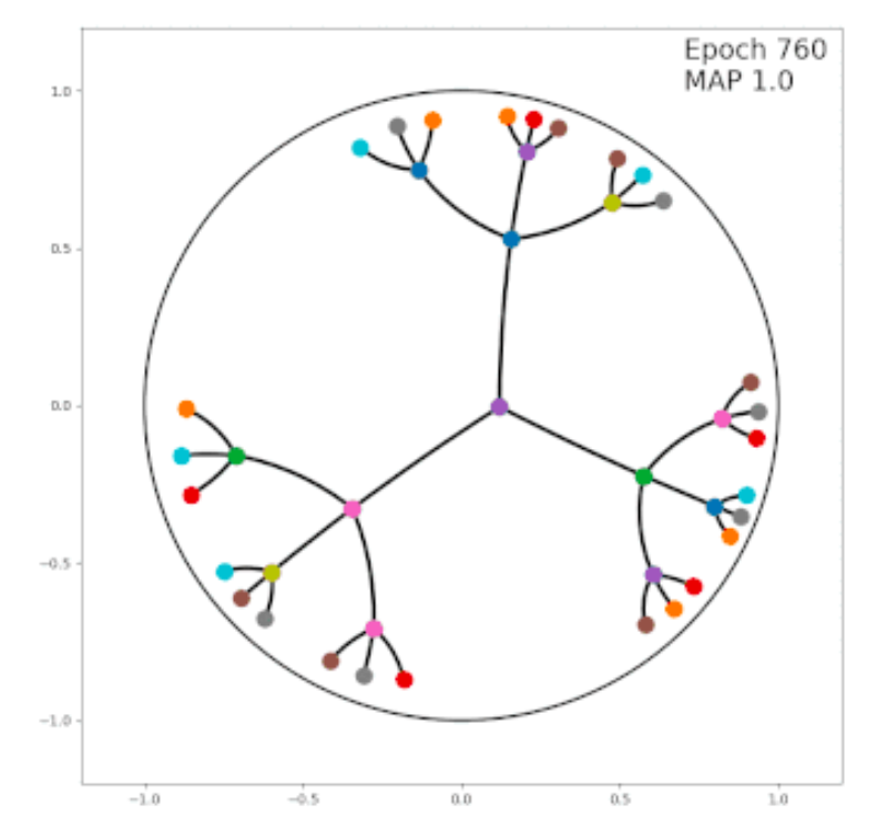
Example 2:

There are hierarchical relationships places like WordNet, Wikipedia categories and knowledge graphs. Exploiting all of these with a machine learning model requires continuous representations, and so we must embed a tree into a continuous space (Graph Embedding). Specifically, we want to maintain the distances of nodes in the tree when these are embedded. Thus we’d like the embedded versions of a pair of sibling nodes to be at distance 2, an embedded node and its parent to be at distance 1, and so on. Ideally, we’d like a ball whose volume grows exponentially in the radius. This doesn’t happen in Euclidean space. But in fact, hyperbolic space offers exactly this property.

Gaussian Embedding

Intuition:

Suppose we have the following text corpus

1. “I was tired.”
2. “I am a student.”
3. “I was studying.”
4. “Am I good at studying?”

and we want to train word embeddings from this corpus. The problem is that words like “I” appears a lot, but words like “good” and “student” only occur once. If a word appears a lot in a corpus, then we would have confidence for the trained word embedding. Conversely, if a word only occur few times, the trained word embedding would have high uncertainty. Usually we have the following way to solve this problem:

• Increse the size of the text corpus.

• Remove words that have frequencies below a threshold.

• Use a sub-word model (split a word into sub-words; this solves the oov (out of vocabulary) problem).

• Learn the uncertainty from the data and add the uncertainty into the word embedding. We call this embedding Gaussian Embedding. For example, we can learn a Gussian Embedding for the word good as $E_{\text{good}} \sim \mathcal{N}(\mu_{\text{good}}, \Sigma_{\text{good}})$

Gaussian Embedding:

An embedded vector representing a point estimate does not naturally express uncertainty about the target concepts with which the input may be associated. Point vectors are typically compared by dot products, cosine-distance or Euclean distance, none of which provide for asymmetric comparisons between objects (as is necessary to represent inclusion or entailment).

In the Gaussian Embedding, both means and variances are learned from the text corpus. Note that Gaussian distributions innately represent uncertainty. If we want to compare two Gaussian word embeddings, since the parameters are distributions, KL-Divergence comes naturally, which is naturally an asymmetric distance meansurement.

Graph Embedding

Definition:

Graph embedding is an approach that is used to transform nodes, edges, and their features into a lower dimensional vector space and whilst maximally preserving properties like graph structure and information.

Because of the complexity of networks, there is no good graph embedding method that can apply to all networks. The embedding approaches vary in performance on different datasets.

node2vec:

There are many graph embedding methods, and a popular one is called node2vec.

Inspired by the Skip-gram model, recent research established an analogy for networks by representing a network as a “document”. The same way as a document is an ordered sequence of words, one could sample sequences of nodes from the underlying network and turn a network into a ordered sequence of nodes.

The node2vec model also introduce the way to make it more flexible to sample nodes from a network.

• It used Breadth-first Sampling (BFS) to obtain a micro-scopic view of the neighborhood of every node and Depth-first Sampling (DFS) to reflect a macro-scopic view of the neighborhood of every node.

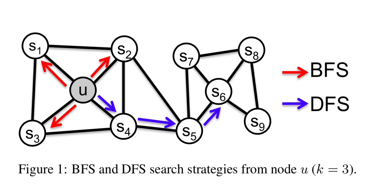
• It also introduced biased random walks, which use parameters $p$ and $q$ to control the weight of BFS and DFS.

I’m going to write a separate post to explain node2vec in detail in the future. Stay tuned!

---

Reference:

• http://ling.umd.edu/~ellenlau/courses/ling646/Plate_2003.pdf
• https://www.quora.com/What-are-the-advantages-of-distributed-representations
• http://www.davidsbatista.net/blog/2018/12/06/Word_Embeddings/
• https://towardsdatascience.com/overview-of-deep-learning-on-graph-embeddings-4305c10ad4a4
• https://www.quora.com/What-is-hierarchical-softmax
• https://dawn.cs.stanford.edu/2019/10/10/noneuclidean/
• https://towardsdatascience.com/overview-of-deep-learning-on-graph-embeddings-4305c10ad4a4
• Vilnis, Luke and McCallum, Andrew. Word representations via gaussian embedding. In ICLR, 2015.
• Aditya Grover and Jure Leskovec. node2vec: Scalable feature learning for networks. In Proceedings of the 22nd ACM SIGKDD International Conference on Knowledge Discovery and Data Mining. ACM, 2016.

往期文章链接目录