第十章 多元分析
第一节 聚类分析
介绍
这里是司守奎教授的《数学建模算法与应用》全书案例代码python实现,欢迎加入此项目将其案例代码用python实现
GitHub项目地址:Mathematical-modeling-algorithm-and-Application
CSDN专栏:数学建模
知乎专栏:数学建模算法与应用
联系作者
作者:STL_CC
邮箱:[email protected]
由于作者还是大一学生,才疏学浅,难免会有错误,欢迎指正
同时作者精力有限,希望更多大佬加入此项目,一来可以提高建模水平,二来可以分享建模经验
系统聚类法
例10.1
设有5个销售员 w 1 w_1 w1, w 2 w_2 w2, w 3 w_3 w3, w 4 w_4 w4, w 5 w_5 w5,他们的销售业绩由二维变量( v 1 v_1 v1, v 2 v_2 v2)描述,见表1 销售员业绩表
| 销售员 | v 1 v_1 v1(销售量)百件 | v 2 v_2 v2(回收款项)万元 |
|---|---|---|
| w 1 w_1 w1 | 1 | 0 |
| w 2 w_2 w2 | 1 | 1 |
| w 3 w_3 w3 | 3 | 2 |
| w 4 w_4 w4 | 4 | 3 |
| w 5 w_5 w5 | 2 | 5 |
方法一 系统聚类法中的最长距离法
import numpy as np
import numpy.matlib
import pandas as pd
import matplotlib
import matplotlib.pyplot as plt
from scipy.spatial.distance import pdist,squareform
from scipy.cluster.hierarchy import dendrogram, linkage,fcluster
a = np.array([[1,0],[1,1],[3,2],[4,3],[2,5]])
(m,n)=a.shape
d = np.zeros((m,m))
for i in range(m):
    for j in range(i+1,m):
        d[i,j]=sum(map(abs,(a[i,:]-a[j,:])))
nd=d.ravel()[np.flatnonzero(d)]
nd=np.unique(nd)
l=len(nd)
for i in range(0,l):
    nd_min=min(nd)
    (row,col)=np.where(d==nd_min)
    tm=np.union1d(row,col)
    print('第{:d}次合成,平台高度为{}时的分类结果为:{}'.format(i+1,nd_min,tm))
    nd=np.delete(nd,np.where(nd==min(nd)))
    if(not len(nd)):
        break
第1次合成,平台高度为1.0时的分类结果为:[0 1]
第2次合成,平台高度为2.0时的分类结果为:[2 3]
第3次合成,平台高度为3.0时的分类结果为:[1 2]
第4次合成,平台高度为4.0时的分类结果为:[0 2 3 4]
第5次合成,平台高度为5.0时的分类结果为:[1 3 4]
第6次合成,平台高度为6.0时的分类结果为:[0 3 4]
方法二 使用python的scipy库
import numpy as np
import pandas as pd
import matplotlib
import matplotlib.pyplot as plt
from scipy.spatial.distance import pdist,squareform
from scipy.cluster.hierarchy import dendrogram, linkage,fcluster
a = np.array([[1,0],[1,1],[3,2],[4,3],[2,5]])
y=pdist(a,'cityblock')
yc=squareform(y)
z=linkage(y)
dendrogram(z)
{'icoord': [[15.0, 15.0, 25.0, 25.0],
  [35.0, 35.0, 45.0, 45.0],
  [20.0, 20.0, 40.0, 40.0],
  [5.0, 5.0, 30.0, 30.0]],
 'dcoord': [[0.0, 1.0, 1.0, 0.0],
  [0.0, 2.0, 2.0, 0.0],
  [1.0, 3.0, 3.0, 2.0],
  [0.0, 4.0, 4.0, 3.0]],
 'ivl': ['4', '0', '1', '2', '3'],
 'leaves': [4, 0, 1, 2, 3],
 'color_list': ['g', 'r', 'b', 'b']}

T = fcluster(z,3,'maxclust')
for i in range(1,3+1):
    tm=np.where(T==i)
    print('第{}类的有'.format(i),tm)
第1类的有 (array([0, 1], dtype=int64),)
第2类的有 (array([2, 3], dtype=int64),)
第3类的有 (array([4], dtype=int64),)
变量聚类法
例10.2 服装标准制定中的变量聚类法。
在服装标准制定中,对某地成年女子的各部位尺寸进行了统计,通过14个部位的测量资料,获得各因素之间的相关系数表(见表5)。
注:具体资料见教材,部分数据将在程序中给出
import numpy as np
import pandas as pd
import matplotlib
import matplotlib.pyplot as plt
from scipy.spatial.distance import pdist,squareform
from scipy.cluster.hierarchy import dendrogram, linkage,fcluster
a=pd.read_csv('ch.txt',header=None,sep=' ')
a
| 0 | 1 | 2 | 3 | 4 | 5 | 6 | 7 | 8 | 9 | 10 | 11 | 12 | 13 | |
|---|---|---|---|---|---|---|---|---|---|---|---|---|---|---|
| 0 | 1.000 | NaN | NaN | NaN | NaN | NaN | NaN | NaN | NaN | NaN | NaN | NaN | NaN | NaN |
| 1 | 0.366 | 1.000 | NaN | NaN | NaN | NaN | NaN | NaN | NaN | NaN | NaN | NaN | NaN | NaN |
| 2 | 0.242 | 0.233 | 1.000 | NaN | NaN | NaN | NaN | NaN | NaN | NaN | NaN | NaN | NaN | NaN |
| 3 | 0.280 | 0.194 | 0.590 | 1.000 | NaN | NaN | NaN | NaN | NaN | NaN | NaN | NaN | NaN | NaN |
| 4 | 0.360 | 0.324 | 0.476 | 0.435 | 1.000 | NaN | NaN | NaN | NaN | NaN | NaN | NaN | NaN | NaN |
| 5 | 0.282 | 0.262 | 0.483 | 0.470 | 0.452 | 1.000 | NaN | NaN | NaN | NaN | NaN | NaN | NaN | NaN |
| 6 | 0.245 | 0.265 | 0.540 | 0.478 | 0.535 | 0.663 | 1.000 | NaN | NaN | NaN | NaN | NaN | NaN | NaN |
| 7 | 0.448 | 0.345 | 0.452 | 0.404 | 0.431 | 0.322 | 0.266 | 1.000 | NaN | NaN | NaN | NaN | NaN | NaN |
| 8 | 0.486 | 0.367 | 0.365 | 0.357 | 0.429 | 0.283 | 0.287 | 0.820 | 1.000 | NaN | NaN | NaN | NaN | NaN |
| 9 | 0.648 | 0.662 | 0.216 | 0.032 | 0.429 | 0.283 | 0.263 | 0.527 | 0.547 | 1.000 | NaN | NaN | NaN | NaN |
| 10 | 0.689 | 0.671 | 0.243 | 0.313 | 0.430 | 0.302 | 0.294 | 0.520 | 0.558 | 0.957 | 1.000 | NaN | NaN | NaN |
| 11 | 0.486 | 0.636 | 0.174 | 0.243 | 0.375 | 0.296 | 0.255 | 0.403 | 0.417 | 0.857 | 0.852 | 1.000 | NaN | NaN |
| 12 | 0.133 | 0.153 | 0.732 | 0.477 | 0.339 | 0.392 | 0.446 | 0.266 | 0.241 | 0.054 | 0.099 | 0.055 | 1.000 | NaN |
| 13 | 0.376 | 0.252 | 0.676 | 0.581 | 0.441 | 0.447 | 0.440 | 0.424 | 0.372 | 0.363 | 0.376 | 0.321 | 0.627 | 1.0 |
d=1-abs(a)
for i in range(len(d)):
    for j in range(i+1,len(d)):
        d.iloc[i,j]=d.iloc[j,i]
z=linkage(d,'complete')
y=fcluster(z,2,'maxclust')
dendrogram(z)
{'icoord': [[25.0, 25.0, 35.0, 35.0],
  [15.0, 15.0, 30.0, 30.0],
  [5.0, 5.0, 22.5, 22.5],
  [55.0, 55.0, 65.0, 65.0],
  [45.0, 45.0, 60.0, 60.0],
  [13.75, 13.75, 52.5, 52.5],
  [85.0, 85.0, 95.0, 95.0],
  [75.0, 75.0, 90.0, 90.0],
  [125.0, 125.0, 135.0, 135.0],
  [115.0, 115.0, 130.0, 130.0],
  [105.0, 105.0, 122.5, 122.5],
  [82.5, 82.5, 113.75, 113.75],
  [33.125, 33.125, 98.125, 98.125]],
 'dcoord': [[0.0, 0.29809729955167313, 0.29809729955167313, 0.0],
  [0.0, 0.4028870809544531, 0.4028870809544531, 0.29809729955167313],
  [0.0, 0.7535436284648688, 0.7535436284648688, 0.4028870809544531],
  [0.0, 0.28955310393777517, 0.28955310393777517, 0.0],
  [0.0, 0.9263082640244553, 0.9263082640244553, 0.28955310393777517],
  [0.7535436284648688,
   1.158768311613672,
   1.158768311613672,
   0.9263082640244553],
  [0.0, 0.49697082409332655, 0.49697082409332655, 0.0],
  [0.0, 0.8415325305655154, 0.8415325305655154, 0.49697082409332655],
  [0.0, 0.5600321419347287, 0.5600321419347287, 0.0],
  [0.0, 0.7182241989796779, 0.7182241989796779, 0.5600321419347287],
  [0.0, 0.850338756026091, 0.850338756026091, 0.7182241989796779],
  [0.8415325305655154,
   1.2178604189314965,
   1.2178604189314965,
   0.850338756026091],
  [1.158768311613672,
   2.1077737070188536,
   2.1077737070188536,
   1.2178604189314965]],
 'ivl': ['1',
  '11',
  '9',
  '10',
  '0',
  '7',
  '8',
  '4',
  '5',
  '6',
  '12',
  '3',
  '2',
  '13'],
 'leaves': [1, 11, 9, 10, 0, 7, 8, 4, 5, 6, 12, 3, 2, 13],
 'color_list': ['g',
  'g',
  'g',
  'g',
  'g',
  'g',
  'r',
  'r',
  'r',
  'r',
  'r',
  'r',
  'b']}

说明
1.在教材原来的matlab程序的数据预处理中,原始数据被去掉了0,向量长度不一。然而这样长度不一的向量是不能在python中被处理的。笔者将其转换为了一个对称矩阵再行操作,更能适应python操作。
2.在matlab中,相关系数矩阵计算使用的corrcoef列指标是变量,然而np.corrcoef行指标是向量,所以要先转置
参考文献
1.python中scipy库实现计算各种距离
2.Python之向量(Vector)距离矩阵计算
3.scipy.spatial.distance.pdist官方文档
4.使用Python进行层次聚类(一)——基本使用+主成分分析绘图观察结果+绘制热图
5.python的scipy层次聚类参数详解
6.皮尔逊积矩相关系数–NumPy–corrcoef()
案例研究
聚类分析案例—我国各地区普通高等教育发展状况分析
具体资料见教材,部分数据将在程序中给出
R型聚类分析

import numpy as np
import pandas as pd
import matplotlib
import matplotlib.pyplot as plt
from scipy.spatial.distance import pdist,squareform
from scipy.cluster.hierarchy import dendrogram, linkage,fcluster
gj=pd.read_csv('gj.txt',header=None,sep=' ').T
r=np.corrcoef(gj)
d=1-r
d=d.T
z=linkage(d,'average')
dendrogram(z)
D:\Program Files\anaconda\lib\site-packages\ipykernel_launcher.py:4: ClusterWarning: scipy.cluster: The symmetric non-negative hollow observation matrix looks suspiciously like an uncondensed distance matrix
  after removing the cwd from sys.path.


{'icoord': [[5.0, 5.0, 15.0, 15.0],
  [55.0, 55.0, 65.0, 65.0],
  [85.0, 85.0, 95.0, 95.0],
  [75.0, 75.0, 90.0, 90.0],
  [60.0, 60.0, 82.5, 82.5],
  [45.0, 45.0, 71.25, 71.25],
  [35.0, 35.0, 58.125, 58.125],
  [25.0, 25.0, 46.5625, 46.5625],
  [10.0, 10.0, 35.78125, 35.78125]],
 'dcoord': [[0.0, 0.8525484864006131, 0.8525484864006131, 0.0],
  [0.0, 0.024863305626884467, 0.024863305626884467, 0.0],
  [0.0, 0.02757546216575882, 0.02757546216575882, 0.0],
  [0.0, 0.04009972160627508, 0.04009972160627508, 0.02757546216575882],
  [0.024863305626884467,
   0.14222971620143948,
   0.14222971620143948,
   0.04009972160627508],
  [0.0, 0.3129510501346711, 0.3129510501346711, 0.14222971620143948],
  [0.0, 0.4732207840475411, 0.4732207840475411, 0.3129510501346711],
  [0.0, 1.0379457746449512, 1.0379457746449512, 0.4732207840475411],
  [0.8525484864006131,
   1.7688040008982475,
   1.7688040008982475,
   1.0379457746449512]],
 'ivl': ['6', '7', '9', '8', '0', '4', '5', '1', '2', '3'],
 'leaves': [6, 7, 9, 8, 0, 4, 5, 1, 2, 3],
 'color_list': ['g', 'r', 'r', 'r', 'r', 'r', 'r', 'r', 'b']}

T=fcluster(z,6,'maxclust')
for i in range(1,6+1):
    tm=np.where(T==i)
    print('第{}类的有'.format(i),tm)
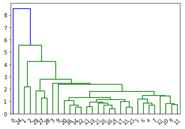
Q型聚类分析
第1类的有 (array([ 1,  2,  5,  6,  9, 14, 16, 20, 22, 27, 28], dtype=int64),)
第2类的有 (array([11, 17, 19], dtype=int64),)
第3类的有 (array([ 3,  4,  7,  8, 10, 12, 13, 15, 18, 23, 25, 26], dtype=int64),)
第4类的有 (array([ 0, 29], dtype=int64),)
第5类的有 (array([24], dtype=int64),)
第6类的有 (array([21], dtype=int64),)
import numpy as np
import pandas as pd
import matplotlib
import matplotlib.pyplot as plt
from scipy.spatial.distance import pdist,squareform
from scipy.cluster.hierarchy import dendrogram, linkage,fcluster
from scipy.stats import zscore
gj=pd.read_csv('gj.txt',header=None,sep='	')
gj.drop([2,3,4,5],axis=1,inplace=True)
gj=zscore(gj)
y=pdist(gj)
z=linkage(y,'average')
dendrogram(z)
{'icoord': [[25.0, 25.0, 35.0, 35.0],
  [55.0, 55.0, 65.0, 65.0],
  [45.0, 45.0, 60.0, 60.0],
  [115.0, 115.0, 125.0, 125.0],
  [105.0, 105.0, 120.0, 120.0],
  [95.0, 95.0, 112.5, 112.5],
  [135.0, 135.0, 145.0, 145.0],
  [175.0, 175.0, 185.0, 185.0],
  [165.0, 165.0, 180.0, 180.0],
  [155.0, 155.0, 172.5, 172.5],
  [140.0, 140.0, 163.75, 163.75],
  [205.0, 205.0, 215.0, 215.0],
  [195.0, 195.0, 210.0, 210.0],
  [151.875, 151.875, 202.5, 202.5],
  [103.75, 103.75, 177.1875, 177.1875],
  [245.0, 245.0, 255.0, 255.0],
  [235.0, 235.0, 250.0, 250.0],
  [225.0, 225.0, 242.5, 242.5],
  [285.0, 285.0, 295.0, 295.0],
  [275.0, 275.0, 290.0, 290.0],
  [265.0, 265.0, 282.5, 282.5],
  [233.75, 233.75, 273.75, 273.75],
  [140.46875, 140.46875, 253.75, 253.75],
  [85.0, 85.0, 197.109375, 197.109375],
  [75.0, 75.0, 141.0546875, 141.0546875],
  [52.5, 52.5, 108.02734375, 108.02734375],
  [30.0, 30.0, 80.263671875, 80.263671875],
  [15.0, 15.0, 55.1318359375, 55.1318359375],
  [5.0, 5.0, 35.06591796875, 35.06591796875]],
 'dcoord': [[0.0, 2.165069616081611, 2.165069616081611, 0.0],
  [0.0, 1.2583609996700658, 1.2583609996700658, 0.0],
  [0.0, 1.8417771551214015, 1.8417771551214015, 1.2583609996700658],
  [0.0, 0.5102264872107092, 0.5102264872107092, 0.0],
  [0.0, 0.6832038743184952, 0.6832038743184952, 0.5102264872107092],
  [0.0, 1.0534720455396414, 1.0534720455396414, 0.6832038743184952],
  [0.0, 0.5781192315086323, 0.5781192315086323, 0.0],
  [0.0, 0.39279767533924836, 0.39279767533924836, 0.0],
  [0.0, 0.6920728341799272, 0.6920728341799272, 0.39279767533924836],
  [0.0, 0.8587702247881565, 0.8587702247881565, 0.6920728341799272],
  [0.5781192315086323,
   0.951351143405573,
   0.951351143405573,
   0.8587702247881565],
  [0.0, 0.5422575852550412, 0.5422575852550412, 0.0],
  [0.0, 0.9931260197301512, 0.9931260197301512, 0.5422575852550412],
  [0.951351143405573,
   1.1337053131831187,
   1.1337053131831187,
   0.9931260197301512],
  [1.0534720455396414,
   1.3091848224406866,
   1.3091848224406866,
   1.1337053131831187],
  [0.0, 0.7003307018910611, 0.7003307018910611, 0.0],
  [0.0, 0.8455264592324916, 0.8455264592324916, 0.7003307018910611],
  [0.0, 1.183614496022609, 1.183614496022609, 0.8455264592324916],
  [0.0, 0.7408663414479949, 0.7408663414479949, 0.0],
  [0.0, 0.7928025480682006, 0.7928025480682006, 0.7408663414479949],
  [0.0, 1.43244903784588, 1.43244903784588, 0.7928025480682006],
  [1.183614496022609,
   1.4564970761510314,
   1.4564970761510314,
   1.43244903784588],
  [1.3091848224406866,
   1.7995913531962198,
   1.7995913531962198,
   1.4564970761510314],
  [0.0, 2.389167635724778, 2.389167635724778, 1.7995913531962198],
  [0.0, 2.4533056587669138, 2.4533056587669138, 2.389167635724778],
  [1.8417771551214015,
   2.801906683718659,
   2.801906683718659,
   2.4533056587669138],
  [2.165069616081611, 4.23103702123038, 4.23103702123038, 2.801906683718659],
  [0.0, 5.540472787063805, 5.540472787063805, 4.23103702123038],
  [0.0, 8.531300289191663, 8.531300289191663, 5.540472787063805]],
 'ivl': ['0',
  '24',
  '1',
  '2',
  '29',
  '27',
  '28',
  '3',
  '9',
  '20',
  '16',
  '14',
  '22',
  '13',
  '19',
  '21',
  '26',
  '18',
  '25',
  '17',
  '15',
  '23',
  '5',
  '6',
  '4',
  '7',
  '12',
  '10',
  '8',
  '11'],
 'leaves': [0,
  24,
  1,
  2,
  29,
  27,
  28,
  3,
  9,
  20,
  16,
  14,
  22,
  13,
  19,
  21,
  26,
  18,
  25,
  17,
  15,
  23,
  5,
  6,
  4,
  7,
  12,
  10,
  8,
  11],
 'color_list': ['g',
  'g',
  'g',
  'g',
  'g',
  'g',
  'g',
  'g',
  'g',
  'g',
  'g',
  'g',
  'g',
  'g',
  'g',
  'g',
  'g',
  'g',
  'g',
  'g',
  'g',
  'g',
  'g',
  'g',
  'g',
  'g',
  'g',
  'g',
  'b']}
for k in range(3,6):
    print('划分成{}类的结果如下'.format(k))
    T=fcluster(z,k,'maxclust')
    for i in range(1,k+1):
        tm=np.where(T==i)
        print('第{}类的有{}'.format(i,tm))
划分成3类的结果如下
第1类的有(array([ 1,  2,  3,  4,  5,  6,  7,  8,  9, 10, 11, 12, 13, 14, 15, 16, 17,
       18, 19, 20, 21, 22, 23, 25, 26, 27, 28, 29], dtype=int64),)
第2类的有(array([24], dtype=int64),)
第3类的有(array([0], dtype=int64),)
划分成4类的结果如下
第1类的有(array([1, 2], dtype=int64),)
第2类的有(array([ 3,  4,  5,  6,  7,  8,  9, 10, 11, 12, 13, 14, 15, 16, 17, 18, 19,
       20, 21, 22, 23, 25, 26, 27, 28, 29], dtype=int64),)
第3类的有(array([24], dtype=int64),)
第4类的有(array([0], dtype=int64),)
划分成5类的结果如下
第1类的有(array([1, 2], dtype=int64),)
第2类的有(array([27, 28, 29], dtype=int64),)
第3类的有(array([ 3,  4,  5,  6,  7,  8,  9, 10, 11, 12, 13, 14, 15, 16, 17, 18, 19,
       20, 21, 22, 23, 25, 26], dtype=int64),)
第4类的有(array([24], dtype=int64),)
第5类的有(array([0], dtype=int64),)