空间平滑MUSIC算法(1)
1. 前言
在上一篇博客中有提到,当多个入射信号相干时,传统MUSIC算法的效果就会不理想。具体原因是多个入射信号相干时,有部分能量就会散发到噪声子空间,使得MUSIC算法不能对其进行有效估计。
针对这种情况,解相干方法被提出。本文主要讲解通过降维处理解相干,之所以叫降维处理是因为这种方法将原阵列拆分成很多个子阵列,通过子阵列的协方差矩阵重构接收数据协方差矩阵,阵列的自由度DOF会随之降低,即可分辨的相干信号数降低。
先看看传统MUSIC算法对相干信号进行DOA估计的效果。
MATLAB代码
% Code For Music Algorithm
% The Signals Are All Coherent
% Author:痒羊羊
% Date:2020/10/29

clc; clear all; close all;
%% -------------------------initialization-------------------------
f = 500;                                        % frequency
c = 1500;                                       % speed sound
lambda = c/f;                                   % wavelength
d = lambda/2;                                   % array element spacing
M = 20;                                         % number of array elements
N = 100;                                        % number of snapshot
K = 6;                                          % number of sources
coef = [1; exp(1i*pi/6);...
        exp(1i*pi/3); exp(1i*pi/2);...
        exp(2i*pi/3); exp(1i*2*pi)];            % coherence coefficient, K*1
doa_phi = [-30, 0, 20, 40, 60, 75];             % direction of arrivals

%% generate signal
dd = (0:M-1)'*d;                                % distance between array elements and reference element
A = exp(-1i*2*pi*dd*sind(doa_phi)/lambda);      % manifold array, M*K
S = sqrt(2)\(randn(1,N)+1i*randn(1,N));         % vector of random signal, 1*N
X = A*(coef*S);                                 % received data without noise, M*N
X = awgn(X,10,'measured');                      % received data with SNR 10dB

%% calculate the covariance matrix of received data and do eigenvalue decomposition
Rxx = X*X'/N;                                   % covariance matrix
[U,V] = eig(Rxx);                               % eigenvalue decomposition
V = diag(V);                                    % vectorize eigenvalue matrix
[V,idx] = sort(V,'descend');                    % sort the eigenvalues in descending order
U = U(:,idx);                                   % reset the eigenvector
P = sum(V);                                     % power of received data
P_cum = cumsum(V);                              % cumsum of V

%% define the noise space
J = find(P_cum/P>=0.95);                        % or the coefficient is 0.9
J = J(1);                                       % number of principal component
Un = U(:,J+1:end);

%% music for doa; seek the peek
theta = -90:0.1:90;                             % steer theta
doa_a = exp(-1i*2*pi*dd*sind(theta)/lambda);    % manifold array for seeking peak
music = abs(diag(1./(doa_a'*(Un*Un')*doa_a)));  % the result of each theta
music = 10*log10(music/max(music));             % normalize the result and convert it to dB

%% plot
figure;
plot(theta, music, 'linewidth', 2);
title('Music Algorithm For Doa', 'fontsize', 16);
xlabel('Theta(°)', 'fontsize', 16);
ylabel('Spatial Spectrum(dB)', 'fontsize', 16);
grid on;
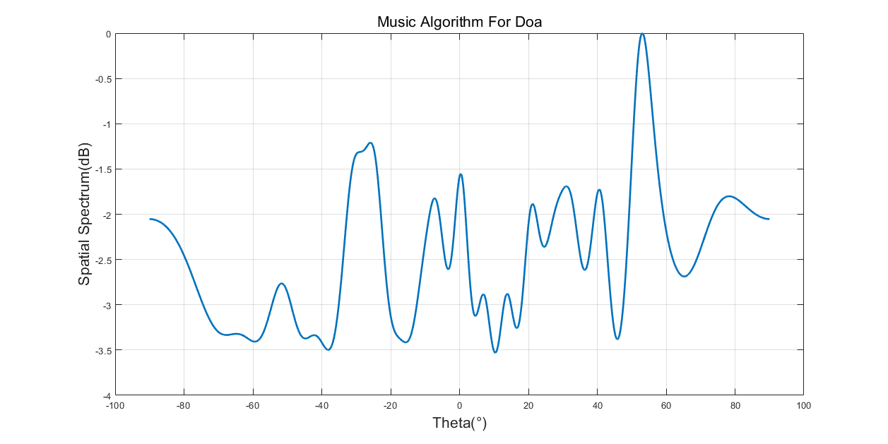
可以看到,对于相干信号,传统MUSIC算法DOA估计效果很差。
2. 空间平滑算法
降维处理解相干方法主要包括空间平滑类处理算法,而空间平滑类处理算法可以分成前向空间平滑算法(FSS)、后向平滑算法(BSS)、前后向平滑算法(FBSS),正如上面所说,这些算法的估计效果很好,但是损失了阵列孔径,导致可分辨的相干信号数降低。
2.1 线性阵列信号模型
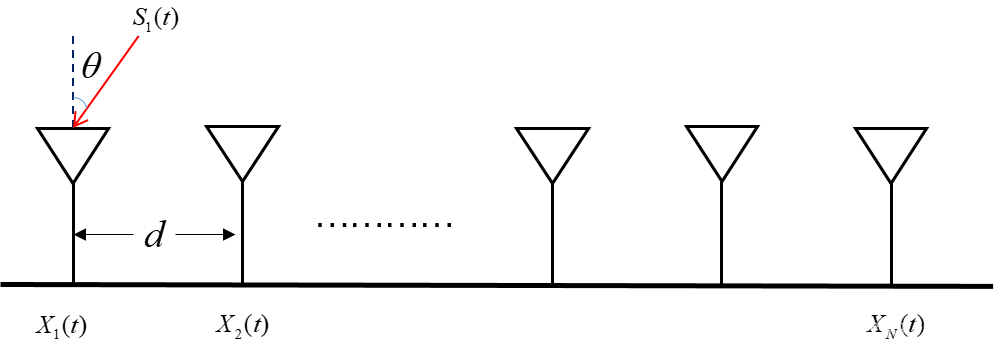
关于这个线性阵列中符号的具体说明可以参考上一篇博文。子空间方法——MUSIC算法
2.2 前向空间平滑算法
前向空间平滑算法将阵列分成多个互相重叠的子阵列,然后对子阵接收数据的协方差矩阵作平均。当子阵阵元数目大于等于相干信号数时,可以有效解相干。
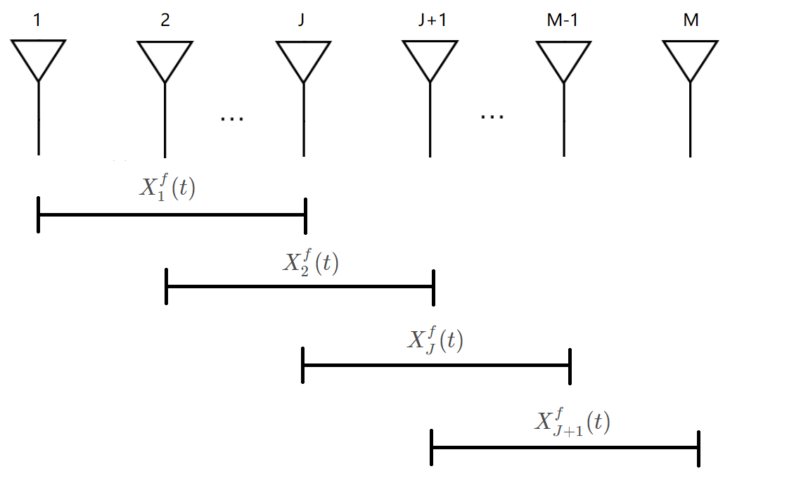
如上图所示,我们把M元阵列均匀分成L个子阵列,每个子阵列有N=M-L+1个阵元。以最左边的子阵列为参考阵列,定义第J个子阵的接收数据为:
X J f = [ x J , x J + 1 , ⋯ , x J + N − 1 ] X_{J}^{f}=\left[x_{J}, x_{J+1}, \cdots, x_{J+N-1}\right] XJf=[xJ,xJ+1,⋯,xJ+N−1]那么第J个子阵接收数据的协方差矩阵(也称作空间平滑矩阵)可以表示为
R N j j = A 1 D j − 1 R s ( D j − 1 ) H A 1 H + σ 2 I N j = 1 , 2 , ⋯ , L R_{N}^{j j}=A_{1} D^{j-1} R_{s}\left(D^{j-1}\right)^{H} A_{1}^{H}+\sigma^{2} I_{N} \quad j=1,2, \cdots, L RNjj=A1Dj−1Rs(Dj−1)HA1H+σ2INj=1,2,⋯,L其中, D = diag [ e − j − 2 π d λ sin θ 1 , e − j 2 π d λ sin θ 2 , ⋯ e − j 2 π d λ sin θ R ] D=\operatorname{diag}\left[\mathrm{e}^{-j\frac{-2 \pi d}{\lambda} \sin \theta_{1}}, \mathrm{e}^{-j\frac{2 \pi d}{\lambda} \sin \theta_{2}}, \cdots \mathrm{e}^{-j\frac{2 \pi d}{\lambda} \sin \theta_{R}}\right] D=diag[e−jλ−2πdsinθ1,e−jλ2πdsinθ2,⋯e−jλ2πdsinθR],A1为第一个子阵即参考阵列的流型矩阵。
因此,前向空间平滑后的协方差矩阵可以由各个子阵的协方差矩阵求平均得到。
R ~ f = 1 L ∑ j = 1 L R N j j \tilde{R}^{f}=\frac{1}{L} \sum_{j=1}^{L} R_{N}^{j j} R~f=L1j=1∑LRNjj利用前向空间平滑协方差矩阵和MUSIC算法就可以分辨出多个相干信号的方位。可以证明,该方法最大可以检测M/2个相干的信号。
MATLAB代码
% Code For Music Algorithm
% The Signals Are All Coherent
% Author:痒羊羊
% Date:2020/10/29

clc; clear all; close all;
%% -------------------------initialization-------------------------
f = 500;                                        % frequency
c = 1500;                                       % speed sound
lambda = c/f;                                   % wavelength
d = lambda/2;                                   % array element spacing
M = 20;                                         % number of array elements
N = 100;                                        % number of snapshot
K = 6;                                          % number of sources
L = 10;                                         % number of subarray
L_N = M-L+1;                                    % number of array elements in each subarray
coef = [1; exp(1i*pi/6);...
        exp(1i*pi/3); exp(1i*pi/2);...
        exp(2i*pi/3); exp(1i*2*pi)];            % coherence coefficient, K*1
doa_phi = [-30, 0, 20, 40, 60, 75];             % direction of arrivals

%% generate signal
dd = (0:M-1)'*d;                                % distance between array elements and reference element
A = exp(-1i*2*pi*dd*sind(doa_phi)/lambda);      % manifold array, M*K
S = sqrt(2)\(randn(1,N)+1i*randn(1,N));         % vector of random signal, 1*N
X = A*(coef*S);                                 % received data without noise, M*N
X = awgn(X,10,'measured');                      % received data with SNR 10dB

%% reconstruct convariance matrix
%% calculate the covariance matrix of received data and do eigenvalue decomposition
Rxx = X*X'/N;                                   % origin covariance matrix
Rf = zeros(L_N, L_N);                           % reconstructed covariance matrix
for i = 1:L
    Rf = Rf+Rxx(i:i+L_N-1,i:i+L_N-1);
end
Rf = Rf/L;
[U,V] = eig(Rf);                                % eigenvalue decomposition
V = diag(V);                                    % vectorize eigenvalue matrix
[V,idx] = sort(V,'descend');                    % sort the eigenvalues in descending order
U = U(:,idx);                                   % reset the eigenvector
P = sum(V);                                     % power of received data
P_cum = cumsum(V);                              % cumsum of V

%% define the noise space
J = find(P_cum/P>=0.95);                        % or the coefficient is 0.9
J = J(1);                                       % number of principal component
Un = U(:,J+1:end);

%% music for doa; seek the peek
dd1 = (0:L_N-1)'*d;
theta = -90:0.1:90;                             % steer theta
doa_a = exp(-1i*2*pi*dd1*sind(theta)/lambda);   % manifold array for seeking peak
music = abs(diag(1./(doa_a'*(Un*Un')*doa_a)));  % the result of each theta
music = 10*log10(music/max(music));             % normalize the result and convert it to dB

%% plot
figure;
plot(theta, music, 'linewidth', 2);
title('Music Algorithm For Doa', 'fontsize', 16);
xlabel('Theta(°)', 'fontsize', 16);
ylabel('Spatial Spectrum(dB)', 'fontsize', 16);
grid on;
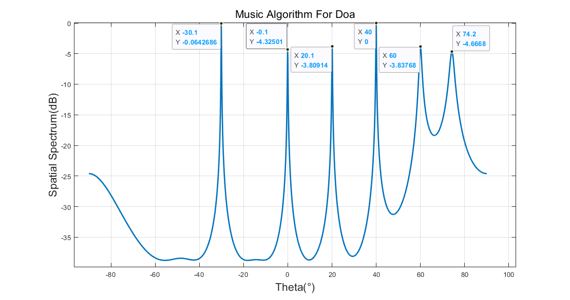
可以看到,在6个入射信号均相干的情况下,基于前向平滑的MUSIC算法能较好地对其进行DOA估计,但仍存在估计精度的问题,比如真实入射角度为75°的信号的方位被估计成了74.2°。
后向空间平滑MUSIC算法和前/后向空间平滑MUSIC算法在下一篇博客中讲解。
参考论文:《基于空间平滑MUSIC算法的相干信号DOA估计,陈文锋,吴桂清》
代码Code均为原创。
欢迎转载,表明出处。