数据分析-学术前沿趋势分析
1 简介
该博客将对于学术前沿论文做一些pandas操作。
1.1 问题背景
本篇博客是对于kaggle里面一个比赛为例子,比赛地址:https://www.kaggle.com/Cornell-University/arxiv,对使用公开的arxiv论文完成一些数据分析操作,实现具体的可视化分析。这篇博客统计2019年全年,计算机各个方向的论文数量。
1.2 数据说明
arXiv 是重要的学术公开网站,也是搜索、浏览和下载学术论文的重要工具。arXiv论文涵盖的范围非常广,涉及物理学的庞大分支和计算机科学的众多子学科,如数学、统计学、电气气工程、定量生物学和经济学等等。数据大小如下图:

2 数据介绍
- 数据集格式如下图:

- 数据集实例:
"root":{


		"id":string"0704.0001"
		"submitter":string"Pavel Nadolsky"
		"authors":string"C. Bal\'azs, E. L. Berger, P. M. Nadolsky, C.-P. Yuan"
		"title":string"Calculation of prompt diphoton production cross sections at Tevatron and LHC energies"
		"comments":string"37 pages, 15 figures; published version"
		"journal-ref":string"Phys.Rev.D76:013009,2007"
		"doi":string"10.1103/PhysRevD.76.013009"
		"report-no":string"ANL-HEP-PR-07-12"
		"categories":string"hep-ph"
		"license":NULL
		"abstract":string"  A fully differential calculation in perturbative quantum chromodynamics is presented for the production of massive photon pairs at hadron colliders. All next-to-leading order perturbative contributions from quark-antiquark, gluon-(anti)quark, and gluon-gluon subprocesses are included, as well as all-orders resummation of initial-state gluon radiation valid at next-to-next-to leading logarithmic accuracy. The region of phase space is specified in which the calculation is most reliable. Good agreement is demonstrated with data from the Fermilab Tevatron, and predictions are made for more detailed tests with CDF and DO data. Predictions are shown for distributions of diphoton pairs produced at the energy of the Large Hadron Collider (LHC). Distributions of the diphoton pairs from the decay of a Higgs boson are contrasted with those produced from QCD processes at the LHC, showing that enhanced sensitivity to the signal can be obtained with judicious selection of events."
		"versions":[
				0:{


						"version":string"v1"
						"created":string"Mon, 2 Apr 2007 19:18:42 GMT"
					}
				1:{


						"version":string"v2"
						"created":string"Tue, 24 Jul 2007 20:10:27 GMT"
					}]
		"update_date":string"2008-11-26"
		"authors_parsed":[
				0:[
						0:string"Balázs"
						1:string"C."
						2:string""]
				1:[
						0:string"Berger"
						1:string"E. L."
						2:string""]
				2:[
						0:string"Nadolsky"
						1:string"P. M."
						2:string""]
				3:[
						0:string"Yuan"
						1:string"C. -P."
						2:string""]]
}
- arxiv论文类别介绍
我们从arxiv官网,查询到论文的类别名称以及其解释如下。
链接:https://arxiv.org/help/api/user-manual 的 5.3 小节的 Subject Classifications 的部分,或 https://arxiv.org/category_taxonomy, 具体的153种paper的类别部分如下:
'astro-ph': 'Astrophysics',
'astro-ph.CO': 'Cosmology and Nongalactic Astrophysics',
'astro-ph.EP': 'Earth and Planetary Astrophysics',
'astro-ph.GA': 'Astrophysics of Galaxies',
'cs.AI': 'Artificial Intelligence',
'cs.AR': 'Hardware Architecture',
'cs.CC': 'Computational Complexity',
'cs.CE': 'Computational Engineering, Finance, and Science',
'cs.CV': 'Computer Vision and Pattern Recognition',
'cs.CY': 'Computers and Society',
'cs.DB': 'Databases',
'cs.DC': 'Distributed, Parallel, and Cluster Computing',
'cs.DL': 'Digital Libraries',
'cs.NA': 'Numerical Analysis',
'cs.NE': 'Neural and Evolutionary Computing',
'cs.NI': 'Networking and Internet Architecture',
'cs.OH': 'Other Computer Science',
'cs.OS': 'Operating Systems',
3 具体代码实现
3.1 导入相关package并读取原始数据
当前环境:Ubuntu18.04+Python3.8+jupyter noteboook
# 导入所需的package
import seaborn as sns #用于画图
from bs4 import BeautifulSoup #用于爬取arxiv的数据
import re #用于正则表达式,匹配字符串的模式
import requests #用于网络连接,发送网络请求,使用域名获取对应信息
import json #读取数据,我们的数据为json格式的
import pandas as pd #数据处理,数据分析
import matplotlib.pyplot as plt #画图工具
接着读入数据
# 读入数据

data  = [] #初始化
#使用with语句优势:1.自动关闭文件句柄;2.自动显示(处理)文件读取数据异常
with open("arxiv-metadata-oai-snapshot.json", 'r') as f:
    for line in f:
        data.append(json.loads(line)) #这里读入的是全部数据,接近18w,可根据需求进行数据的读写

data = pd.DataFrame(data) #将list变为dataframe格式,方便使用pandas进行分析
data.shape #显示数据大小
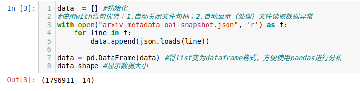
其中的1796911表示数据总量,14表示特征数,也就是之前所说的id什么的。
下面我们看一下该数据集的前5行,用head()函数。这里只截图了一少部分,右边的行数还有部分未截。

对数据进行读入后,接下来就是数据预处理。
3.2 数据预处理
首先先初略统计一下论文的种类信息:

这个结果表明:共有1796911个数据,有62055个子类(因为有论文的类别是多个,例如一篇paper的类别是CS.AI & CS.MM和一篇paper的类别是CS.AI & CS.OS属于不同的子类别,这里仅仅是粗略统计),其中最多的种类是astro-ph,即Astrophysics(天体物理学),共出现了86914次。
由于部分论文的类别不止一种,所以下面我们判断在本数据集中共出现了多少种独立的数据集。

这里使用了 split 函数将多类别使用 “ ”(空格)分开,组成list,并使用 for 循环将独立出现的类别找出来,并使用 set 类别,将重复项去除得到最终所有的独立paper种类。
从以上结果发现,共有176种论文种类,比我们直接从 https://arxiv.org/help/api/user-manual 的 5.3 小节的 Subject Classifications 的部分或 https://arxiv.org/category_taxonomy中的到的类别少,这说明存在一些官网上没有的类别,这是一个小细节。不过对于我们的计算机方向的论文没有影响,依然是以下的40个类别,我们从原数据中提取的和从官网的到的种类是可以一一对应的。
'cs.AI': 'Artificial Intelligence',
'cs.AR': 'Hardware Architecture',
'cs.CC': 'Computational Complexity',
'cs.CE': 'Computational Engineering, Finance, and Science',
'cs.CG': 'Computational Geometry',
'cs.CL': 'Computation and Language',
'cs.CR': 'Cryptography and Security',
'cs.CV': 'Computer Vision and Pattern Recognition',
'cs.CY': 'Computers and Society',
'cs.DB': 'Databases',
'cs.DC': 'Distributed, Parallel, and Cluster Computing',
'cs.DL': 'Digital Libraries',
'cs.DM': 'Discrete Mathematics',
'cs.DS': 'Data Structures and Algorithms',
'cs.ET': 'Emerging Technologies',
'cs.FL': 'Formal Languages and Automata Theory',
'cs.GL': 'General Literature',
'cs.GR': 'Graphics',
'cs.GT': 'Computer Science and Game Theory',
'cs.HC': 'Human-Computer Interaction',
'cs.IR': 'Information Retrieval',
'cs.IT': 'Information Theory',
'cs.LG': 'Machine Learning',
'cs.LO': 'Logic in Computer Science',
'cs.MA': 'Multiagent Systems',
'cs.MM': 'Multimedia',
'cs.MS': 'Mathematical Software',
'cs.NA': 'Numerical Analysis',
'cs.NE': 'Neural and Evolutionary Computing',
'cs.NI': 'Networking and Internet Architecture',
'cs.OH': 'Other Computer Science',
'cs.OS': 'Operating Systems',
'cs.PF': 'Performance',
'cs.PL': 'Programming Languages',
'cs.RO': 'Robotics',
'cs.SC': 'Symbolic Computation',
'cs.SD': 'Sound',
'cs.SE': 'Software Engineering',
'cs.SI': 'Social and Information Networks',
'cs.SY': 'Systems and Control',
对于2019年以后的paper进行分析,所以首先对于时间特征进行预处理,从而得到2019年以后的所有种类的论文:
data["year"] = pd.to_datetime(data["update_date"]).dt.year #将update_date从例如2019-02-20的str变为datetime格式,并提取处year
del data["update_date"] #删除 update_date特征,其使命已完成
data = data[data["year"] >= 2019] #找出 year 中2019年以后的数据,并将其他数据删除
# data.groupby(['categories','year']) #以 categories 进行排序,如果同一个categories 相同则使用 year 特征进行排序
data.reset_index(drop=True, inplace=True) #重新编号
data #查看结果

这里我们就已经得到了所有2019年以后的论文,下面我们挑选出计算机领域内的所有文章:
#爬取所有的类别
website_url = requests.get('https://arxiv.org/category_taxonomy').text #获取网页的文本数据
soup = BeautifulSoup(website_url,'lxml') #爬取数据,这里使用lxml的解析器,加速
root = soup.find('div',{

    'id':'category_taxonomy_list'}) #找出 BeautifulSoup 对应的标签入口
tags = root.find_all(["h2","h3","h4","p"], recursive=True) #读取 tags

#初始化 str 和 list 变量
level_1_name = ""
level_2_name = ""
level_2_code = ""
level_1_names = []
level_2_codes = []
level_2_names = []
level_3_codes = []
level_3_names = []
level_3_notes = []

#进行
for t in tags:
    if t.name == "h2":
        level_1_name = t.text
        level_2_code = t.text
        level_2_name = t.text
    elif t.name == "h3":
        raw = t.text
        level_2_code = re.sub(r"(.*)\((.*)\)",r"\2",raw) #正则表达式:模式字符串:(.*)\((.*)\);被替换字符串"\2";被处理字符串:raw
        level_2_name = re.sub(r"(.*)\((.*)\)",r"\1",raw)
    elif t.name == "h4":
        raw = t.text
        level_3_code = re.sub(r"(.*) \((.*)\)",r"\1",raw)
        level_3_name = re.sub(r"(.*) \((.*)\)",r"\2",raw)
    elif t.name == "p":
        notes = t.text
        level_1_names.append(level_1_name)
        level_2_names.append(level_2_name)
        level_2_codes.append(level_2_code)
        level_3_names.append(level_3_name)
        level_3_codes.append(level_3_code)
        level_3_notes.append(notes)

#根据以上信息生成dataframe格式的数据
df_taxonomy = pd.DataFrame({


    'group_name' : level_1_names,
    'archive_name' : level_2_names,
    'archive_id' : level_2_codes,
    'category_name' : level_3_names,
    'categories' : level_3_codes,
    'category_description': level_3_notes

})

#按照 "group_name" 进行分组,在组内使用 "archive_name" 进行排序
df_taxonomy.groupby(["group_name","archive_name"])
df_taxonomy

3.3 数据分析及可视化
接下来首先看一下所有大类的paper数量分布:
_df = data.merge(df_taxonomy, on="categories", how="left").drop_duplicates(["id","group_name"]).groupby("group_name").agg({

    "id":"count"}).sort_values(by="id",ascending=False).reset_index()

_df
使用merge函数,以两个dataframe共同的属性 “categories” 进行合并,并以 “group_name” 作为类别进行统计,统计结果放入 “id” 列中并排序。

接着我们使用饼图进行上图结果的可视化:
fig = plt.figure(figsize=(15,12))
explode = (0, 0, 0, 0.2, 0.3, 0.3, 0.2, 0.1)
plt.pie(_df["id"],  labels=_df["group_name"], autopct='%1.2f%%', startangle=160, explode=explode)
plt.tight_layout()
plt.show()

下面统计在计算机各个子领域2019年后的paper数量:
group_name="Computer Science"
cats = data.merge(df_taxonomy, on="categories").query("group_name == @group_name")
cats.groupby(["year","category_name"]).count().reset_index().pivot(index="category_name", columns="year",values="id")
我们同样使用 merge 函数,对于两个dataframe 共同的特征 categories 进行合并并且进行查询。然后我们再对于数据进行统计和排序从而得到以下的结果:

总结
我们可以从结果看出,Computer Vision and Pattern Recognition(计算机视觉与模式识别)类是CS中paper数量最多的子类,遥遥领先于其他的CS子类,并且paper的数量还在逐年增加;另外,Computation and Language(计算与语言)、Cryptography and Security(密码学与安全)以及 Robotics(机器人学)的2019年paper数量均超过1000或接近1000,这与我们的认知是一致的。