各位同学好,今天和大家分享一下使用 Tensorflow 构建 DenseNet 卷积神经网络模型,并使用预训练模型的权重,完成对四种天气图片的分类。
完整代码在我的 Gitee 中,有需要的自取:
https://gitee.com/dgvv4/image-classification/tree/master
1. DenseNet
1. 网络介绍
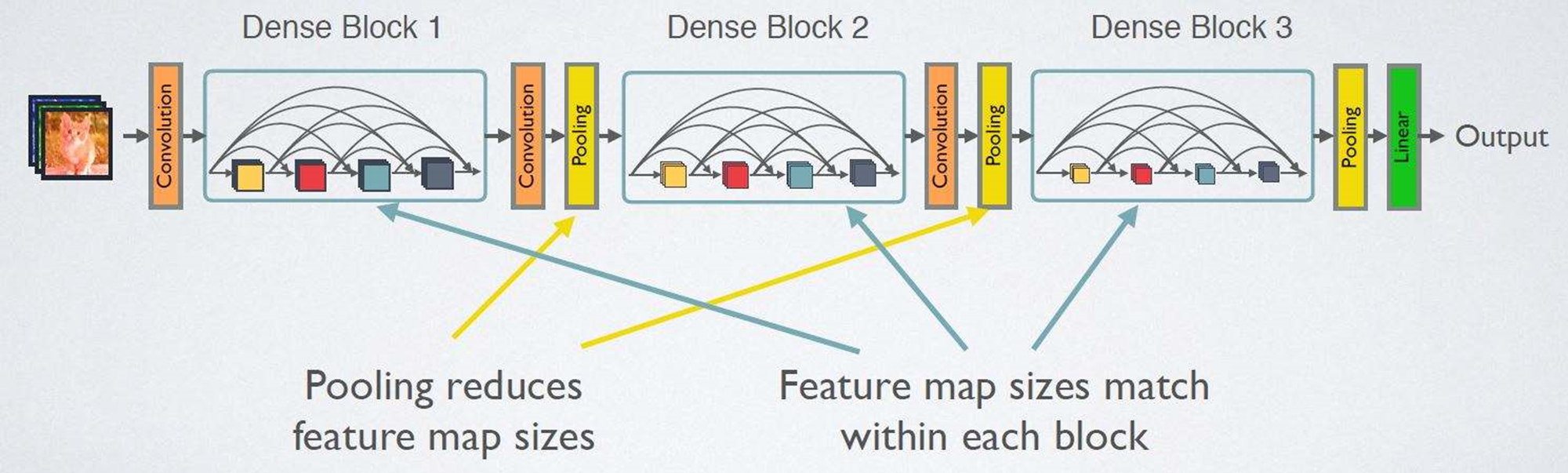
DenseNet 采用密集连接机制,即互相连接的所有层,每个层都会与前面所有层在通道维度上堆叠(layers.Concate),实现特征重用,作为下一层的输入。这样,不但缓解了梯度消失的现象,也使其可以在参与计算量更少的情况下实现比 ResNet 更优的性能。

DenseNet 的密集连接方式需要特征图大小保持一致,所以 DenseNet 网络中使用 DenseBlock + Transition 的结构。DenseBlock 是包含很多层的模块,每个层特征图大小相同,层与层之间采用密集连接方式。Transition模块是连接两个相邻的DenseBlock,并且通过池化层完成下采样。
1.2 DenseBlock代码复现
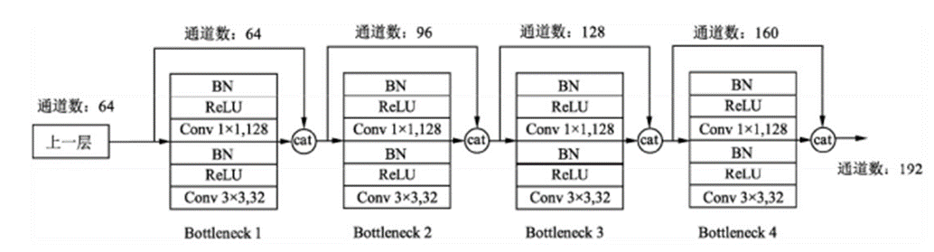
假定输入层的特征图的通道数为 k0,且DenseBlock中各层卷积输出特征图的通道数为 k。那么第L层的输入特征图的通道数是 k0+(L-1)k,我们将k成为网络的增长率(growth_rate)
因为每一层都接收前面的所有层的特征图,即特征传递方式是直接将前面所有层的特征图堆叠(layers.Concate)传到下一层。
DenseBlock 采用激活函数在前,卷积层在后的顺序,即BN+ReLU+Conv的顺序,在DenseNet中该排序方法网络的性能较好。
DenseBlock 内部采用了1*1卷积减少参数量,将前面层的堆叠的通道数下降为4*k个,降低特征输了,提高计算效率。
代码展示:
#(1)构建一个dense单元
def DenseLayer(x, growth_rate, dropout_rate=0.2):

    # BN+激活+1*1卷积降维
    x = layers.BatchNormalization()(x)
    x = layers.Activation('relu')(x)
    x = layers.Conv2D(filters = growth_rate*4,  # 降低特征图数量
                      kernel_size = (1,1),
                      strides = 1,
                      padding = 'same')(x)

    # BN+激活+3*3卷积
    x = layers.BatchNormalization()(x)
    x = layers.Activation('relu')(x)
    x = layers.Conv2D(filters = growth_rate,
                      kernel_size = (3,3),
                      strides = 1,
                      padding = 'same')(x)

    # 随机杀死神经元
    x = layers.Dropout(rate = dropout_rate)(x)

    return x

#(2)构建DenseBlock的多个卷积组合在一起的卷积块
def DenseBlock(x, num, growth_rate):

    # 重复执行多少次DenseLayer
    for _ in range(num):
        conv = DenseLayer(x, growth_rate)
        # 将前面所有层的特征堆叠后传到下一层
        x = layers.Concatenate()([x, conv])

    return x
1.3 Transition 代码展示
Transition 模块主要连接两个相邻的 DenseBlock,并下采样降低特征图的size,压缩模型。Transition层包含一个1*1卷积层和2*2平均池化层。
#(3)Transition层连接两个相邻的DenseBlock
def Transition(x, compression_rate=0.5):

    # 1*1卷积下降一半的通道数
    out_channel = int(x.shape[-1] * compression_rate)

    # BN+激活+1*1卷积+2*2平均池化
    x = layers.BatchNormalization()(x)
    x = layers.Activation('relu')(x)
    x = layers.Conv2D(filters = out_channel,  # 输出通道数
                      kernel_size = (1,1),
                      strides = 1,
                      padding = 'same')(x)
    x = layers.AveragePooling2D(pool_size = (2,2),
                                strides = 2,  # 下采样
                                padding = 'same')(x)
    return x
1.4 构造主干网络
网络结构图如下,我以 DenseNet121 为例构建网络骨干。

#(4)主干网络架构
def densenet(input_shape, classes, growth_rate, include_top):

    # 构造输入层[224,224,3]
    inputs = keras.Input(shape=input_shape)

    # 卷积下采样[224,224,3]==>[112,112,64]
    x = layers.Conv2D(filters = 2*growth_rate,  # 输出特征图个数为两倍增长率
                      kernel_size = (7,7),
                      strides = 2,
                      padding = 'same')(inputs)

    x = layers.BatchNormalization()(x)
    x = layers.Activation('relu')(x)

    # 最大池化[112,112,64]==>[56,56,64]
    x = layers.MaxPooling2D(pool_size = (3,3),
                            strides = 2,
                            padding = 'same')(x)

    # [56,56,64]==>[56,56,64+6*32]
    x = DenseBlock(x, num=6,  growth_rate=growth_rate)
    # [56,56,256]==>[28,28,128]
    x = Transition(x)
    # [28,28,128]==>[28,28,128+12*32]
    x = DenseBlock(x, num=12, growth_rate=growth_rate)
    # [28,28,512]==>[14,14,256]
    x = Transition(x)
    # [14,14,256]==>[14,14,256+24*32]
    x = DenseBlock(x, num=24, growth_rate=growth_rate)
    # [14,14,1024]==>[7,7,512]
    x = Transition(x)
    # [7,7,512]==>[7,7,512+16*32]
    x = DenseBlock(x, num=16, growth_rate=growth_rate)

    # 导入模型时,是否包含输出层
    if include_top is True:

        # [7,7,1024]==>[None,1024]
        x = layers.GlobalAveragePooling2D()(x)
        # [None,1024]==>[None,classes]
        x = layers.Dense(classes)(x)  # 不经过softmax层转换成概率

    # 构造模型
    model = Model(inputs, x)

    return model

#(5)接收网络模型
if __name__ == '__main__':

    model = densenet(input_shape=[224,224,3],  # 输入图像的shape
                     classes = 1000,  # 分类数
                     growth_rate = 32,  # 设置增长率,即每个dense模块的输出通道数
                     include_top = True)  # 默认包含输出层

    model.summary()  # 查看网络架构
2. 网络训练
2.1 加载数据集
函数 tf.keras.preprocessing.image_dataset_from_directory() 构造数据集,
分批次读取图片数据,参数 img_size 会对读进来的图片resize成指定大小;参数 label_mode 中,'int'代表目标值y是数值类型索引,即0, 1, 2, 3等;'categorical'代表onehot类型,对应正确类别的索引的值为1,如图像属于第二类则表示为0,1,0,0,0;'binary'代表二分类。
#(1)加载数据集
def get_data(height, width, batchsz):

    # 训练集数据
    train_ds = keras.preprocessing.image_dataset_from_directory(
        directory = filepath + 'train',  # 训练集图片所在文件夹
        label_mode = 'categorical',  # onehot编码
        image_size = (height, width),  # 输入图象的size
        batch_size = batchsz)  # 每批次训练32张图片

    # 验证集数据
    val_ds = keras.preprocessing.image_dataset_from_directory(
        directory = filepath + 'val',
        label_mode = 'categorical',
        image_size = (height, width),
        batch_size = batchsz)

    # 返回划分好的数据集
    return train_ds, val_ds

# 读取数据集
train_ds, val_ds = get_data(height, width, batchsz)

#(2)查看数据集信息
def check_data(train_ds):  # 传入训练集数据集

    # 查看数据集有几个分类类别
    class_names = train_ds.class_names
    print('classNames:', class_names)

    # 查看数据集的shape, x代表图片数据, y代表分类类别数据
    sample = next(iter(train_ds))  # 生成迭代器,每次取出一个batch的数据
    print('x_batch.shape:', sample[0].shape, 'y_batch.shape:', sample[1].shape)
    print('前五个目标值:', sample[1][:5])

# 是否查看数据集信息
if checkData is True:
    check_data(train_ds)

#(3)查看图像
def plot_show(train_ds):

    # 生成迭代器,每次取出一个batch的数据
    sample = next(iter(train_ds))  # sample[0]图像信息, sample[1]标签信息
    # 显示前5张图
    for i in range(5):
        plt.subplot(1,5,i+1)  # 在一块画板的子画板上绘制1行5列
        plt.imshow(sample[0][i]/255.0)  # 图像的像素值压缩到0-1
        plt.xticks([])  # 不显示xy坐标刻度
        plt.yticks([])
    plt.show()

# 是否展示图像信息
if plotShow is True:
    plot_show(train_ds)
天气图片如下:

2.2 预处理改进
本篇使用迁移学习的方法,使用 DenseNet121 预训练模型的权重训练网络,大体流程和上一篇文章的非迁移学习训练方法类似,这里只说明一下需要改动的地方。可见上一篇案例:https://blog.csdn.net/dgvv4/article/details/123714507
首先,既然使用了别人训练好的权重继续训练,那就要使用和别人一样的数据预处理方法。
在imgnet中数据的预处理方法是,输入图像的各个通道的像素值都减去其均值,不使用像素值归一化的方法。
# 数据预处理不使用归一化,调整RGB三通道颜色均值
_R_MEAN = 123.68
_G_MEAN = 116.78
_B_MEAN = 103.94

#(4)数据预处理
def processing(x,y):  # 定义预处理函数
    x = tf.cast(x, dtype=tf.float32) # 图片转换为tensor类型
    y = tf.cast(y, dtype=tf.int32)  # 分类标签转换成tensor类型
    # 对图像的各个通道减去均值,不进行归一化
    x = x - [_R_MEAN, _G_MEAN, _B_MEAN]

    return x,y

# 对所有数据预处理
train_ds = train_ds.map(processing).shuffle(10000)  # map调用自定义预处理函数, shuffle打乱数据集
val_ds = val_ds.map(processing)
2.3 加载模型和权重
其次,加载网络模型及权重,我们只需要网络的特征提取层,不需要网络的输出层(原网络输出一般都是1000分类)。通过设置 model.trainable = False 就能冻结网络特征提取层的所有权重,正反向传播过程中只有输出层的权重会发生优化更新。建议前10轮的训练冻结特征提取层,后面的训练再设置 model.trainable = True 网络所有权重都能更新。
自定义输出层,由于原网络的输出层一般都是1000分类,而我们自己的网络一般是几个分类,因此输出层的网络结构需要我们自己写。通过 keras.Sequential() 容器堆叠网络各层。
model = densenet(input_shape=input_shape, # 网络的输入图像的size
                classes=classes,  # 分类数
                growth_rate = 32,  # 设置增长率,即每个dense模块的输出通道数
                include_top=False)  # 不载入输出层

# 报错解决:You are trying to load a weight file containing 242 layers into a model with
# 添加参数:by_name=True
model.load_weights(pre_weights_path, by_name=True)

# False冻结模型的所有参数,只能更新输出层的参数
model.trainable = True

# 自定义输出层,不经过softmax激活,有利于网络的稳定性
model = keras.Sequential([model,  # [7,7,1024]
                          layers.GlobalAveragePooling2D(), # ==>[None,1024]
                          layers.Dropout(rate=0.5),
                          layers.Dense(512),  # ==>[None,512]
                          layers.Dropout(rate=0.5),
                          layers.Dense(classes)])  #==>[None,classes]
2.4 训练结果
和非迁移学习的训练方法相比需要改进的部分只有上面两点,接下来开始训练,设置回调函数将验证集损失最低的一次迭代的权重保存下来。
#(7)保存权重文件
if not os.path.exists(weights_dir):  # 判断当前文件夹下有没有一个叫save_weights的文件夹
    os.makedirs(weights_dir)  # 如果没有就创建一个


#(8)模型编译
opt = optimizers.Adam(learning_rate=learning_rate)  # 设置Adam优化器

model.compile(optimizer=opt, #学习率
              loss=keras.losses.CategoricalCrossentropy(from_logits=True), # 交叉熵损失,logits层先经过softmax
              metrics=['accuracy']) #评价指标


#(9)定义回调函数,一个列表
# 保存模型参数
callbacks = [keras.callbacks.ModelCheckpoint(filepath = 'save_weights/densenet.h5',  # 参数保存的位置
                                            save_best_only = True,  # 保存最佳参数
                                            save_weights_only = True,  # 只保存权重文件
                                            monitor = 'val_loss')]  # 通过验证集损失判断是否是最佳参数


#(10)模型训练,history保存训练信息
history = model.fit(x = train_ds,  # 训练集
                    validation_data = val_ds,  # 验证集
                    epochs = epochs,  #迭代30次
                    callbacks = callbacks,
                    initial_epoch=0)
训练完成后,history中保存了训练信息,绘制损失曲线和准确率曲线。
#(11)获取训练信息
history_dict = history.history  # 获取训练的数据字典
train_loss = history_dict['loss']  # 训练集损失
train_accuracy = history_dict['accuracy']  # 训练集准确率
val_loss = history_dict['val_loss']  # 验证集损失
val_accuracy = history_dict['val_accuracy']  # 验证集准确率

#(12)绘制训练损失和验证损失
plt.figure()
plt.plot(range(epochs), train_loss, label='train_loss')  # 训练集损失
plt.plot(range(epochs), val_loss, label='val_loss')  # 验证集损失
plt.legend()  # 显示标签
plt.xlabel('epochs')
plt.ylabel('loss')

#(13)绘制训练集和验证集准确率
plt.figure()
plt.plot(range(epochs), train_accuracy, label='train_accuracy')  # 训练集准确率
plt.plot(range(epochs), val_accuracy, label='val_accuracy')  # 验证集准确率
plt.legend()
plt.xlabel('epochs')
plt.ylabel('accuracy')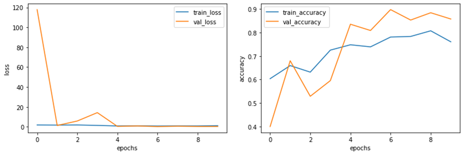
训练过程中的准确率和损失
Epoch 1/10
99/99 [==============================] - 64s 354ms/step - loss: 1.8832 - accuracy: 0.5543 - val_loss: 117.8199 - val_accuracy: 0.4000
Epoch 2/10
99/99 [==============================] - 16s 140ms/step - loss: 1.5482 - accuracy: 0.6619 - val_loss: 1.3441 - val_accuracy: 0.6800
Epoch 3/10
99/99 [==============================] - 16s 138ms/step - loss: 2.0702 - accuracy: 0.6129 - val_loss: 5.8502 - val_accuracy: 0.5289
Epoch 4/10
99/99 [==============================] - 16s 137ms/step - loss: 1.2101 - accuracy: 0.7477 - val_loss: 14.2739 - val_accuracy: 0.5956
Epoch 5/10
99/99 [==============================] - 15s 137ms/step - loss: 0.7785 - accuracy: 0.7687 - val_loss: 0.4700 - val_accuracy: 0.8356
Epoch 6/10
99/99 [==============================] - 16s 138ms/step - loss: 1.1095 - accuracy: 0.7349 - val_loss: 0.8931 - val_accuracy: 0.8089
Epoch 7/10
99/99 [==============================] - 16s 138ms/step - loss: 0.8705 - accuracy: 0.7835 - val_loss: 0.2821 - val_accuracy: 0.8978
Epoch 8/10
99/99 [==============================] - 16s 138ms/step - loss: 0.9680 - accuracy: 0.7760 - val_loss: 0.6360 - val_accuracy: 0.8533
Epoch 9/10
99/99 [==============================] - 16s 139ms/step - loss: 0.9522 - accuracy: 0.8041 - val_loss: 0.3987 - val_accuracy: 0.8844
Epoch 10/10
99/99 [==============================] - 16s 138ms/step - loss: 1.0262 - accuracy: 0.7649 - val_loss: 0.4000 - val_accuracy: 0.8578
3. 预测阶段
以对整个测试集的图片预测为例,test_ds 存放测试集的图片和类别标签,对测试集进行和训练集相同的预处理方法,将图片的每个通道像素值减去每个通道的均值。
model.predict(img) 返回的是每张图片属于每个类别的概率,需要找到概率最大值所对应的索引 np.argmax(result),该索引对应的分类名称就是最终预测结果。
import tensorflow as tf
from tensorflow import keras
from DenseNet import densenet
from PIL import Image
import numpy as np
import matplotlib.pyplot as plt

# 报错解决:NotFoundError: No algorithm worked! when using Conv2D
from tensorflow.compat.v1 import ConfigProto
from tensorflow.compat.v1 import InteractiveSession
config = ConfigProto()
config.gpu_options.allow_growth = True
session = InteractiveSession(config=config)


# ------------------------------------ #
# 预测参数设置
# ------------------------------------ #
im_height = 224  # 输入图像的高
im_width = 224   # 输入图像的高
# 分类名称
class_names = ['cloudy', 'rain', 'shine', 'sunrise']
# 权重路径
weight_dir = 'save_weights/densenet_new.h5'
# ------------------------------------ #
# 数据预处理,调整RGB三通道颜色均值
# ------------------------------------ #
_R_MEAN = 123.68
_G_MEAN = 116.78
_B_MEAN = 103.94
# ------------------------------------ #
# 单张图片预测
# ------------------------------------ #
# 是否只预测一张图
single_pic = False
# 图像所在文件夹的路径
single_filepath = 'D:/deeplearning/test/....../001.jpg'
# 指定某张图片
picture = single_filepath + 'rain94.jpg'

# ------------------------------------ #
# 对测试集图片预测
# ------------------------------------ #
test_pack = True
# 验证集文件夹路径
test_filepath = 'D:/deeplearning/test/数据集/...../test/'


#(1)载入模型,不载入输出层
model = densenet(input_shape=[224,224,3], classes=4, growth_rate = 32, include_top=False)
print('model is loaded')

#(2)构造输出层
model = keras.Sequential([model,
                          keras.layers.GlobalAveragePooling2D(), # ==>[None,1024]
                          keras.layers.Dropout(rate=0.5),
                          keras.layers.Dense(512),  # ==>[None,512]
                          keras.layers.Dropout(rate=0.5),
                          keras.layers.Dense(len(class_names)),  #==>[None,classes]
                          keras.layers.Softmax()])  # 这里需要经过得到softmax分类概率

#(3)载入权重.h文件
model.load_weights(weight_dir, by_name=True)
print('weights is loaded')


#(4)只对单张图像预测
if single_pic is True:

    # 加载图片
    img = Image.open(picture)
    # 改变图片size
    img = img.resize((im_height, im_width))
    # 展示图像
    plt.figure()
    plt.imshow(img)
    plt.xticks([])
    plt.yticks([])

    # 预处理,图像像素值减去均值
    img = np.array(img).astype(np.float32)  # 变成tensor类型
    img = img - [_R_MEAN, _G_MEAN, _B_MEAN]

    # 输入网络的要求,给图像增加一个batch维度, [h,w,c]==>[b,h,w,c]
    img = np.expand_dims(img, axis=0)

    # 预测图片,返回结果包含batch维度[b,n]
    result = model.predict(img)
    # 转换成一维,挤压掉batch维度
    result = np.squeeze(result)

    # 找到概率最大值对应的索引
    predict_class = np.argmax(result)

    # 打印预测类别及概率
    print('class:', class_names[predict_class],
          'prob:', result[predict_class])

    plt.title(f'{class_names[predict_class]}')
    plt.show()

#(5)对测试集图像预测
if test_pack is True:

    # 载入测试集
    test_ds = keras.preprocessing.image_dataset_from_directory(
        directory = test_filepath,
        label_mode = 'int',  # 不经过ont编码, 1、2、3、4、、、
        image_size = (im_height, im_width),  # 测试集的图像resize
        batch_size = 32)  # 每批次32张图

    # 测试集预处理
    #(2)数据预处理
    def processing(image, label):

        image = tf.cast(image, tf.float32)  # 修改数据类型
        label = tf.cast(label, tf.int32)
        # 对图像的各个通道减去均值,不进行归一化
        image = image - [_R_MEAN, _G_MEAN, _B_MEAN]

        return (image, label)

    test_ds = test_ds.map(processing) # 预处理


    test_true = []  # 存放真实值
    test_pred = []  # 存放预测值

    # 遍历测试集所有的batch
    for imgs, labels in test_ds:
        # 每次每次取出一个batch的一张图像和一个标签
        for img, label in zip(imgs, labels):

            # 网络输入的要求,给图像增加一个维度[h,w,c]==>[b,h,w,c]
            image_array = tf.expand_dims(img, axis=0)
            # 预测某一张图片,返回图片属于许多类别的概率
            prediction = model.predict(image_array)

            # 找到预测概率最大的索引对应的类别
            test_pred.append(class_names[np.argmax(prediction)])
            # label是真实标签索引
            test_true.append(class_names[label])

    # 展示结果
    print('真实值: ', test_true[:10])
    print('预测值: ', test_pred[:10])

    # 绘制混淆矩阵
    from sklearn.metrics import confusion_matrix
    import seaborn as sns
    import pandas as pd
    plt.rcParams['font.sans-serif'] = ['SimSun']  #宋体
    plt.rcParams['font.size'] = 15  #设置字体大小

    # 生成混淆矩阵
    conf_numpy = confusion_matrix(test_true, test_pred)
    # 转换成DataFrame表格类型,设置行列标签
    conf_df = pd.DataFrame(conf_numpy, index=class_names, columns=class_names)

    # 创建绘图区
    plt.figure(figsize=(8,7))

    # 生成热力图
    sns.heatmap(conf_df, annot=True, fmt="d", cmap="BuPu")

    # 设置标签
    plt.title('Confusion_Matrix')
    plt.xlabel('Predict')
    plt.ylabel('True')