翻译: 3.6. 从零开始实现 Softmax 回归 pytorch

就像我们从头开始实现线性回归一样，我们相信 softmax 回归同样是基本的，你应该知道它的血腥细节以及如何自己实现它。我们将使用刚刚在第 3.5 节中介绍的 Fashion-MNIST 数据集，设置批量大小为 256 的数据迭代器。

import torch
from IPython import display
from d2l import torch as d2l

batch_size = 256
train_iter, test_iter = d2l.load_data_fashion_mnist(batch_size)

3.6.1. 初始化模型参数
与我们的线性回归示例一样，这里的每个示例都将由一个固定长度的向量表示。原始数据集中的每个示例都是28 x 28图片。在本节中，我们将展平每个图像，将它们视为长度为 784 的向量。将来，我们将讨论更复杂的策略来利用图像中的空间结构，但现在我们将每个像素位置视为另一个特征。

回想一下，在 softmax 回归中，我们有与类一样多的输出。因为我们的数据集有 10 个类别，所以我们的网络的输出维度为 10。因此，我们的权重将构成784 x 10 矩阵和偏差将构成一个1 x 10 行向量。与线性回归一样，我们将W使用高斯噪声和偏差初始化权重以取初始值 0。

num_inputs = 784
num_outputs = 10

W = torch.normal(0, 0.01, size=(num_inputs, num_outputs), requires_grad=True)
b = torch.zeros(num_outputs, requires_grad=True)

3.6.2. 定义 Softmax 操作

在实现 softmax 回归模型之前，让我们简要回顾一下 sum 运算符如何沿张量中的特定维度工作，如第 2.3.6节和 第 2.3.6.1节中讨论的那样。给定一个矩阵X，我们可以对所有元素求和（默认情况下）或仅对同一轴上的元素求和，即同一列（轴 0）或同一行（轴 1）。请注意，如果X是一个形状为 (2, 3) 的张量，并且我们对列求和，则结果将是一个形状为 (3,) 的向量。在调用 sum 运算符时，我们可以指定保留原始张量中的轴数，而不是折叠我们求和的维度。这将产生一个形状为 (1, 3) 的二维张量。

X = torch.tensor([[1.0, 2.0, 3.0], [4.0, 5.0, 6.0]])
X.sum(0, keepdim=True), X.sum(1, keepdim=True)

(tensor([[5., 7., 9.]]),
 tensor([[ 6.],
         [15.]]))

我们现在准备实现 softmax 操作。回想一下，softmax 由三个步骤组成：

• （i）我们对每个项求幂（使用exp）；
• (ii) 我们对每一行求和（批处理中每个示例有一行）以获得每个示例的归一化常数；
• (iii) 我们将每一行除以其归一化常数，确保结果总和为 1。在查看代码之前，让我们回顾一下它是如何表示为一个等式的：
  
  分母或归一化常数有时也称为 分区函数（其对数称为对数分区函数）。该名称的起源是在统计物理学 中，其中一个相关的方程模拟了粒子集合的分布。

def softmax(X):
    X_exp = torch.exp(X)
    partition = X_exp.sum(1, keepdim=True)
    return X_exp / partition  # The broadcasting mechanism is applied here

如您所见，对于任何随机输入，我们将每个元素转换为非负数。此外，每一行总和为 1，这是概率所必需的。

X = torch.normal(0, 1, (2, 5))
X_prob = softmax(X)
X_prob, X_prob.sum(1)

(tensor([[0.0622, 0.1872, 0.1356, 0.2527, 0.3623],
         [0.1034, 0.1495, 0.3899, 0.3203, 0.0369]]),
 tensor([1., 1.]))

请注意，虽然这在数学上看起来是正确的，但我们在实现中有点草率，因为我们未能采取预防措施来防止由于矩阵的大或非常小的元素而导致的数值溢出或下溢。

3.6.3. 定义模型

现在我们已经定义了 softmax 操作，我们可以实现 softmax 回归模型了。下面的代码定义了输入如何通过网络映射到输出。请注意，reshape在将数据传递给我们的模型之前，我们使用该函数将批次中的每个原始图像展平为一个向量。

def net(X):
    return softmax(torch.matmul(X.reshape((-1, W.shape[0])), W) + b)

3.6.4. 定义损失函数

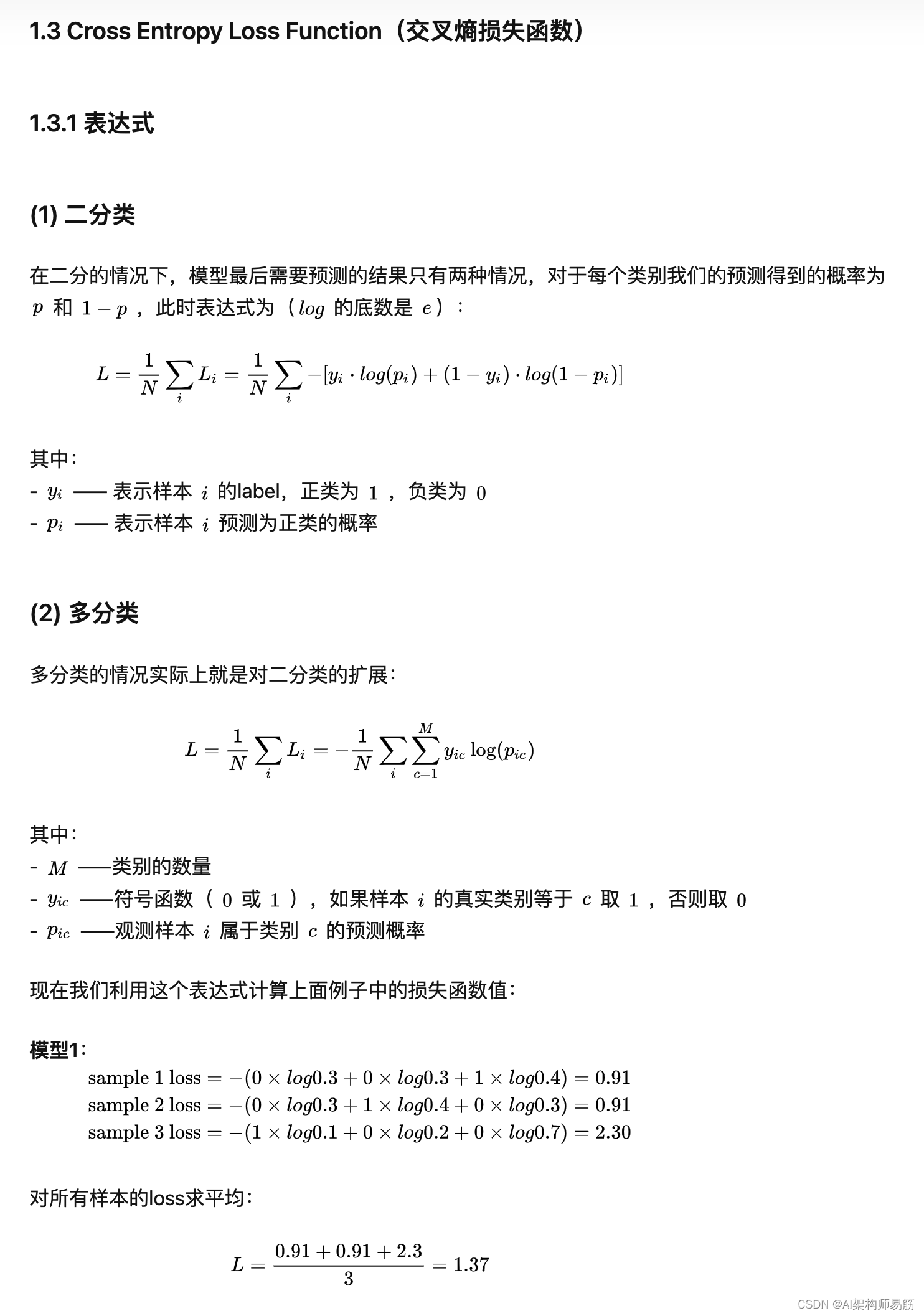
接下来，我们需要实现3.4 节中介绍的交叉熵损失函数。这可能是所有深度学习中最常见的损失函数，因为目前分类问题的数量远远超过回归问题。

回想一下，交叉熵采用分配给真实标签的预测概率的负对数似然。我们可以通过一个运算符来选择所有元素，而不是使用 Python for 循环（这往往效率低下）来迭代预测。下面，我们创建样本数据y_hat，其中包含 3 个类别的预测概率的 2 个示例及其对应的标签y。我们知道，在y第一个例子中，第一个值是正确的预测，在第二个例子中，第三个值是真实的。使用y 中的概率指标y_hat，我们选择第一个示例中第一类的概率和第二个示例中第三类的概率。

y = torch.tensor([0, 2])
y_hat = torch.tensor([[0.1, 0.3, 0.6], [0.3, 0.2, 0.5]])
y_hat[[0, 1], y]

tensor([0.1000, 0.5000])

现在我们只需一行代码就可以有效地实现交叉熵损失函数。

def cross_entropy(y_hat, y):
    return - torch.log(y_hat[range(len(y_hat)), y])

cross_entropy(y_hat, y)

tensor([2.3026, 0.6931])

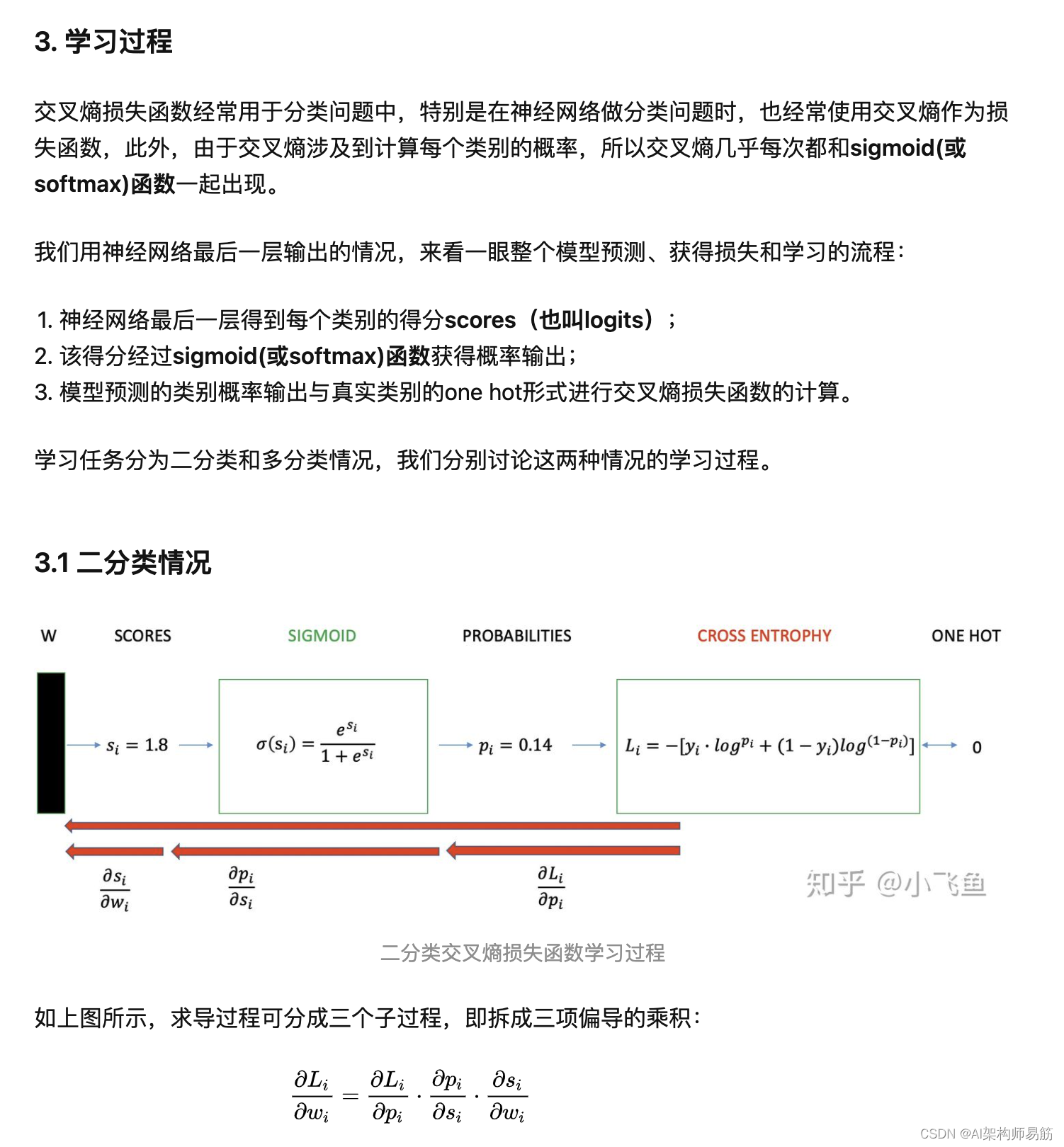
ground true 的意思是正确答案的意思。
比如 arr = [0.3, 0.2, 0.5]的ground true最大概率是arr[1]
图片例子请看下图。

3.6.5。分类精度

给定预测概率分布y_hat，我们通常在必须输出硬预测时选择预测概率最高的类。事实上，许多应用程序需要我们做出选择。Gmail 必须将电子邮件分类为“首要”、“社交”、“更新”或“论坛”。它可能会在内部估计概率，但最终它必须在类中选择一个。

当预测与标签类一致时y，它们是正确的。分类准确度是所有预测正确的部分。虽然直接优化准确率可能很困难（它不可微），但它通常是我们最关心的性能指标，我们几乎总是会在训练分类器时报告它。

为了计算准确性，我们执行以下操作。首先，如果y_hat是一个矩阵，我们假设第二个维度存储每个类别的预测分数。我们使用argmax每行中最大条目的索引来获取预测类。然后我们将预测的类与基本事实y元素进行比较。由于相等运算符 ==对数据类型敏感，我们将y_hat的数据类型转换为与 的匹配y。结果是一个包含 0（假）和 1（真）条目的张量。取总和得出正确预测的数量。

def accuracy(y_hat, y):  #@save
    """Compute the number of correct predictions."""
    if len(y_hat.shape) > 1 and y_hat.shape[1] > 1:
        y_hat = y_hat.argmax(axis=1)
    cmp = y_hat.type(y.dtype) == y
    return float(cmp.type(y.dtype).sum())

我们将继续使用之前定义的变量y_hat和变量分别作为预测的概率分布和标签。y我们可以看到第一个例子的预测类是2（行的最大元素是0.6，索引是2），预测值0和实际的标签不一致。第二个例子的预测类是2（行的最大元素为0.5，索引为2)，与实际标签2一致。因此，这两个示例的分类准确率为0.5。

accuracy(y_hat, y) / len(y)

0.5

同样，我们可以在通过数据迭代器访问的数据集上评估任何模型net的准确性

def evaluate_accuracy(net, data_iter):  #@save
    """Compute the accuracy for a model on a dataset."""
    if isinstance(net, torch.nn.Module):
        net.eval()  # Set the model to evaluation mode
    metric = Accumulator(2)  # No. of correct predictions, no. of predictions

    with torch.no_grad():
        for X, y in data_iter:
            metric.add(accuracy(net(X), y), y.numel())
    return metric[0] / metric[1]

这Accumulator是一个程序类，用于累积多个变量的总和。在上面的evaluate_accuracy函数中，我们在Accumulator实例中创建了 2 个变量，分别用于存储正确预测的数量和预测的数量。当我们迭代数据集时，两者都会随着时间的推移而累积。

class Accumulator:  #@save
    """For accumulating sums over `n` variables."""
    def __init__(self, n):
        self.data = [0.0] * n

    def add(self, *args):
        self.data = [a + float(b) for a, b in zip(self.data, args)]

    def reset(self):
        self.data = [0.0] * len(self.data)

    def __getitem__(self, idx):
        return self.data[idx]

因为我们net用随机权重初始化模型，所以这个模型的准确率应该接近随机猜测，即 10 类为 0.1。

evaluate_accuracy(net, test_iter)

0.0967

3.6.6。训练

如果您通读 第 3.2 节中的线性回归实现，softmax 回归的训练循环应该看起来非常熟悉。在这里，我们重构实现以使其可重用。首先，我们定义一个函数来训练一个 epoch。请注意，这updater是一个更新模型参数的通用函数，它接受批量大小作为参数。它可以是d2l.sgd函数的包装器，也可以是框架的内置优化函数。

def train_epoch_ch3(net, train_iter, loss, updater):  #@save
    """The training loop defined in Chapter 3."""
    # Set the model to training mode
    if isinstance(net, torch.nn.Module):
        net.train()
    # Sum of training loss, sum of training accuracy, no. of examples
    metric = Accumulator(3)
    for X, y in train_iter:
        # Compute gradients and update parameters
        y_hat = net(X)
        l = loss(y_hat, y)
        if isinstance(updater, torch.optim.Optimizer):
            # Using PyTorch in-built optimizer & loss criterion
            updater.zero_grad()
            l.mean().backward()
            updater.step()
        else:
            # Using custom built optimizer & loss criterion
            l.sum().backward()
            updater(X.shape[0])
        metric.add(float(l.sum()), accuracy(y_hat, y), y.numel())
    # Return training loss and training accuracy
    return metric[0] / metric[2], metric[1] / metric[2]

在展示训练函数的实现之前，我们定义了一个以动画形式绘制数据的实用程序类。同样，它旨在简化本书其余部分的代码。

class Animator:  #@save
    """For plotting data in animation."""
    def __init__(self, xlabel=None, ylabel=None, legend=None, xlim=None,
                 ylim=None, xscale='linear', yscale='linear',
                 fmts=('-', 'm--', 'g-.', 'r:'), nrows=1, ncols=1,
                 figsize=(3.5, 2.5)):
        # Incrementally plot multiple lines
        if legend is None:
            legend = []
        d2l.use_svg_display()
        self.fig, self.axes = d2l.plt.subplots(nrows, ncols, figsize=figsize)
        if nrows * ncols == 1:
            self.axes = [self.axes, ]
        # Use a lambda function to capture arguments
        self.config_axes = lambda: d2l.set_axes(
            self.axes[0], xlabel, ylabel, xlim, ylim, xscale, yscale, legend)
        self.X, self.Y, self.fmts = None, None, fmts

    def add(self, x, y):
        # Add multiple data points into the figure
        if not hasattr(y, "__len__"):
            y = [y]
        n = len(y)
        if not hasattr(x, "__len__"):
            x = [x] * n
        if not self.X:
            self.X = [[] for _ in range(n)]
        if not self.Y:
            self.Y = [[] for _ in range(n)]
        for i, (a, b) in enumerate(zip(x, y)):
            if a is not None and b is not None:
                self.X[i].append(a)
                self.Y[i].append(b)
        self.axes[0].cla()
        for x, y, fmt in zip(self.X, self.Y, self.fmts):
            self.axes[0].plot(x, y, fmt)
        self.config_axes()
        display.display(self.fig)
        display.clear_output(wait=True)

然后，以下训练函数net在一个训练数据集上训练一个模型，该训练数据集通过train_iter指定的多个 epoch访问num_epochs。在每个 epoch 结束时，模型在通过 访问的测试数据集上进行评估test_iter。我们将利用Animator课程来可视化培训进度。

def train_ch3(net, train_iter, test_iter, loss, num_epochs, updater):  #@save
    """Train a model (defined in Chapter 3)."""
    animator = Animator(xlabel='epoch', xlim=[1, num_epochs], ylim=[0.3, 0.9],
                        legend=['train loss', 'train acc', 'test acc'])
    for epoch in range(num_epochs):
        train_metrics = train_epoch_ch3(net, train_iter, loss, updater)
        test_acc = evaluate_accuracy(net, test_iter)
        animator.add(epoch + 1, train_metrics + (test_acc,))
    train_loss, train_acc = train_metrics
    assert train_loss < 0.5, train_loss
    assert train_acc <= 1 and train_acc > 0.7, train_acc
    assert test_acc <= 1 and test_acc > 0.7, test_acc

作为从头开始的实现，我们使用第 3.2 节中定义的小批量随机梯度下降来优化模型的损失函数，学习率为 0.1。

lr = 0.1

def updater(batch_size):
    return d2l.sgd([W, b], lr, batch_size)

现在我们用 10 个 epoch 训练模型。请注意，时期数 ( num_epochs) 和学习率 ( lr) 都是可调整的超参数。通过改变它们的值，我们或许能够提高模型的分类精度。

num_epochs = 10
train_ch3(net, train_iter, test_iter, cross_entropy, num_epochs, updater)

3.6.7. 预测

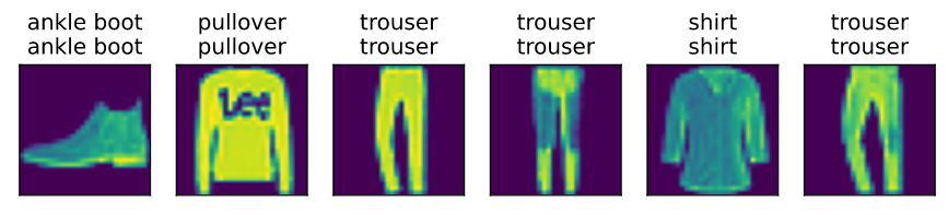
现在训练已经完成，我们的模型已经准备好对一些图像进行分类了。给定一系列图像，我们将比较它们的实际标签（第一行文本输出）和模型的预测（第二行文本输出）。

def predict_ch3(net, test_iter, n=6):  #@save
    """Predict labels (defined in Chapter 3)."""
    for X, y in test_iter:
        break
    trues = d2l.get_fashion_mnist_labels(y)
    preds = d2l.get_fashion_mnist_labels(net(X).argmax(axis=1))
    titles = [true +'\n' + pred for true, pred in zip(trues, preds)]
    d2l.show_images(
        X[0:n].reshape((n, 28, 28)), 1, n, titles=titles[0:n])

predict_ch3(net, test_iter)

3.6.8。概括

使用 softmax 回归，我们可以训练模型进行多类分类。

softmax 回归的训练循环与线性回归非常相似：检索和读取数据，定义模型和损失函数，然后使用优化算法训练模型。您很快就会发现，大多数常见的深度学习模型都有类似的训练过程。

3.6.9。练习

1. 在本节中，我们根据 softmax 操作的数学定义直接实现了 softmax 函数。这可能会导致什么问题？提示：尝试计算大小exp(50) .

Nothing happened!? And, max number of 64float is 2^1024 - 2^(1023-52).
So e^1024 will overflow？

X = torch.tensor([[500., 510., 520.], [540., 550., 560.]])
X_prob = softmax(X)
X_prob

tensor([[nan, nan, nan],
        [nan, nan, nan]])

2. 本节中的函数cross_entropy是根据交叉熵损失函数的定义来实现的。这个实现可能有什么问题？提示：考虑对数的域。
   log(0) will error!

3. 您能想到什么解决方案来解决上述两个问题？
   先经过sigmoid，使得所有概率值都在(0,1)之间，再做softmax处理。
   

4. 返回最有可能的标签总是一个好主意吗？例如，您会为医疗诊断这样做吗？
   In medical diagnosis, we may more need to find all possible result to avoid condition worsening.

5. 假设我们要使用 softmax 回归根据一些特征来预测下一个词。大词汇量可能会出现哪些问题？
   A large vocabulary will make every word’s probabilty near to 0.

参考

https://d2l.ai/chapter_linear-networks/softmax-regression-scratch.html
https://www.zhihu.com/question/22464082
https://zhuanlan.zhihu.com/p/35709485