一、Matlab小波分析往期经典推文超链接:
3 《中国七大气候分区》
5 《Matlab 小波功率谱》
6 《水文模型—Matlab版本(1)》

二、Python小波分析:
源代码和数据来自克里斯·托伦斯博士github:
https://github.com/chris-torrence
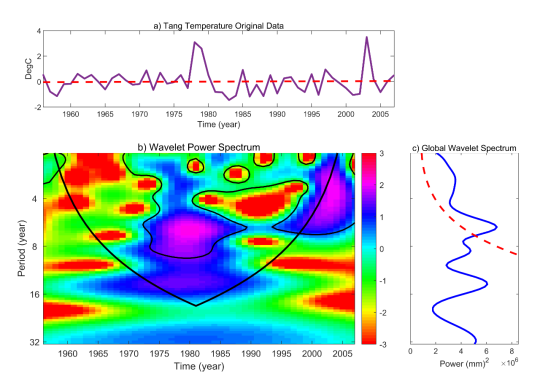
import numpy as npfrom waveletFunctions import wavelet, wave_signifimport matplotlib.pylab as pltfrom matplotlib.gridspec import GridSpecimport matplotlib.ticker as tickerfrom mpl_toolkits.axes_grid1 import make_axes_locatable__author__ = 'Evgeniya Predybaylo'## READ THE DATAsst = np.loadtxt('F:/Rpython/lp28/data/sst_nino3.dat') # input SST time seriessst = sst - np.mean(sst)variance = np.std(sst, ddof=1) ** 2print("variance = ", variance)if 0:variance = 1.0sst = sst / np.std(sst, ddof=1)n = len(sst)dt = 0.25time = np.arange(len(sst)) * dt + 1871.0 # construct time arrayxlim = ([1870, 2000]) # plotting rangepad = 1 # pad the time series with zeroes (recommended)dj = 0.25 # this will do 4 sub-octaves per octaves0 = 2 * dt # this says start at a scale of 6 monthsj1 = 7 / dj # this says do 7 powers-of-two with dj sub-octaves eachlag1 = 0.72 # lag-1 autocorrelation for red noise backgroundprint("lag1 = ", lag1)mother = 'MORLET'# Wavelet transform:wave, period, scale, coi = wavelet(sst, dt, pad, dj, s0, j1, mother)power = (np.abs(wave)) ** 2 # compute wavelet power spectrumglobal_ws = (np.sum(power, axis=1) / n) # time-average over all times# Significance levels:signif = wave_signif(([variance]), dt=dt, sigtest=0, scale=scale,lag1=lag1, mother=mother)sig95 = signif[:, np.newaxis].dot(np.ones(n)[np.newaxis, :]) # expand signif --> (J+1)x(N) arraysig95 = power / sig95 # where ratio > 1, power is significant# Global wavelet spectrum & significance levels:dof = n - scale # the -scale corrects for padding at edgesglobal_signif = wave_signif(variance, dt=dt, scale=scale, sigtest=1,lag1=lag1, dof=dof, mother=mother)# Scale-average between El Nino periods of 2--8 yearsavg = np.logical_and(scale >= 2, scale < 8)Cdelta = 0.776 # this is for the MORLET waveletscale_avg = scale[:, np.newaxis].dot(np.ones(n)[np.newaxis, :]) # expand scale --> (J+1)x(N) arrayscale_avg = power / scale_avg # [Eqn(24)]scale_avg = dj * dt / Cdelta * sum(scale_avg[avg, :]) # [Eqn(24)]scaleavg_signif = wave_signif(variance, dt=dt, scale=scale, sigtest=2,lag1=lag1, dof=([2, 7.9]), mother=mother)#--- Plot time seriesfig = plt.figure(figsize=(9, 10))gs = GridSpec(3, 4, hspace=0.4, wspace=0.75)plt.subplots_adjust(left=0.1, bottom=0.05, right=0.9, top=0.95, wspace=0, hspace=0)plt.subplot(gs[0, 0:3])plt.plot(time, sst, 'k')plt.xlim(xlim[:])plt.xlabel('Time (year)')plt.ylabel('NINO3 SST (\u00B0C)')plt.title('a) NINO3 Sea Surface Temperature (seasonal)')plt.text(time[-1] + 35, 0.5,'Wavelet Analysis\nC. Torrence & G.P. Compo\n' +'http://paos.colorado.edu/\nresearch/wavelets/',horizontalalignment='center', verticalalignment='center')#--- Contour plot wavelet power spectrum# plt3 = plt.subplot(3, 1, 2)plt3 = plt.subplot(gs[1, 0:3])levels = [0, 0.5, 1, 2, 4, 999]CS = plt.contourf(time, period, power, len(levels)) #*** or use 'contour'im = plt.contourf(CS, levels=levels, colors=['white','bisque','orange','orangered','darkred'])plt.xlabel('Time (year)')plt.ylabel('Period (years)')plt.title('b) Wavelet Power Spectrum (contours at 0.5,1,2,4\u00B0C$^2$)')plt.xlim(xlim[:])# 95# significance contour, levels at -99 (fake) and 1 (95# signif)plt.contour(time, period, sig95, [-99, 1], colors='k')# cone-of-influence, anything "below" is dubiousplt.plot(time, coi, 'k')# format y-scaleplt3.set_yscale('log', basey=2, subsy=None)plt.ylim([np.min(period), np.max(period)])ax = plt.gca().yaxisax.set_major_formatter(ticker.ScalarFormatter())plt3.ticklabel_format(axis='y', style='plain')plt3.invert_yaxis()plt4 = plt.subplot(gs[1, -1])plt.plot(global_ws, period)plt.plot(global_signif, period, '--')plt.xlabel('Power (\u00B0C$^2$)')plt.title('c) Global Wavelet Spectrum')plt.xlim([0, 1.25 * np.max(global_ws)])# format y-scaleplt4.set_yscale('log', basey=2, subsy=None)plt.ylim([np.min(period), np.max(period)])ax = plt.gca().yaxisax.set_major_formatter(ticker.ScalarFormatter())plt4.ticklabel_format(axis='y', style='plain')plt4.invert_yaxis()# --- Plot 2--8 yr scale-average time seriesplt.subplot(gs[2, 0:3])plt.plot(time, scale_avg, 'k')plt.xlim(xlim[:])plt.xlabel('Time (year)')plt.ylabel('Avg variance (\u00B0C$^2$)')plt.title('d) 2-8 yr Scale-average Time Series')plt.plot(xlim, scaleavg_signif + [0, 0], '--')plt.savefig('F:/Rpython/lp28/plot27.png',dpi=1200)plt.show()

三、Kriging、IDW空间插值上期推文超链接:
《Matlab克里金(Kriging)、反距离权重(IDW)空间插值》
