1、Kaggle比赛 - 泰坦尼克号
泰坦尼克号的沉没是历史上最著名的沉船事件之一。1912 年 4 月 15 日,在她的处女航中,泰坦尼克号在与冰山相撞后沉没,2224 名乘客和船员中有 1502 人遇难。这一耸人听闻的悲剧震惊了国际社会,并导致了更好的船舶安全法规。
沉船事故导致生命损失的原因之一是没有足够的救生艇供乘客和船员使用。尽管在沉没中幸存下来有一些运气成分,但某些人群比其他人群更有可能幸存下来,例如妇女、儿童和上层阶级。
在这个挑战中,我们要求您完成对什么样的人可能幸存下来的分析。特别是,我们要求您应用机器学习工具来预测哪些乘客在这场悲剧中幸存下来。
比赛网址,数据集也从这个页面下载
 https://www.kaggle.com/competitions/titanic/overview
2、数据集介绍
历史数据分为两组,“训练集”和“测试集”。对于训练集,我们为每位乘客提供结果(“ground truth”)。您将使用此集来构建模型以生成测试集的预测。
对于测试集中的每位乘客,您必须预测他们是否在沉船中幸存下来(0 表示已故,1 表示幸存)。您的分数是您正确预测的乘客百分比。
Kaggle 排行榜分为公共和私有。您对测试集的 50% 预测已随机分配到公共排行榜(所有用户的 50% 相同)。您在此公开部分的得分将显示在排行榜上。比赛结束时,我们将在私密的 50% 数据上公布您的得分,这将决定最终获胜者。此方法可防止用户“过度拟合”排行榜。
数据集部分数据如下
其中
Survived:(0 = No; 1 = Yes)
Pclass:客舱等级(1 = 1 级;2 = 2 级;3 = 3 级)
Name:姓名
Sex:性别
Age:年龄
SibSp:船上的兄弟姐妹/配偶人数
Parch:船上的父母/儿童人数,有些孩子只和保姆一起旅行,因此他们的parch=0。
Ticket:票号
Fare:票价
Cabin:客舱号
Embarked:登船港口,C = 瑟堡,Q = 皇后镇,S = 南安普顿
3、数据探索性分析
(1)导入包
import pandas as pd
import numpy as np
import pylab as plt

# 设置 matplotlib 图形的全局默认大小
plt.rc('figure', figsize=(10, 5))

# 包含子图的 matplotlib 图形的大小
fizsize_with_subplots = (10, 10)

# matplotlib 直方图箱的大小
bin_size = 10
(2)读取数据
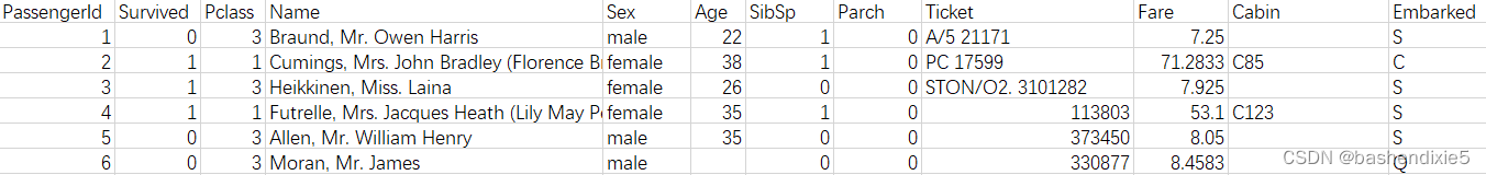
df_train = pd.read_csv('../data/titanic/train.csv')
df_train.head()
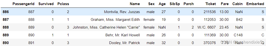
df_train.tail()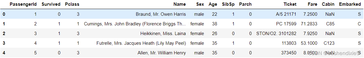
(3)查看列的数据类型
df_train.dtypes信息如下
[5 rows x 12 columns]
PassengerId      int64
Survived         int64
Pclass           int64
Name            object
Sex             object
Age            float64
SibSp            int64
Parch            int64
Ticket          object
Fare           float64
Cabin           object
Embarked        object
dtype: object
类型 'object' 是 pandas 的字符串,它不适合机器学习算法。 如果我们想将这些用作特征,我们需要将它们转换为数字表示。
(4)获取DataFrame的基本信息
df_train.info()基本信息如下
<class 'pandas.core.frame.DataFrame'>
RangeIndex: 891 entries, 0 to 890
Data columns (total 12 columns):
 #   Column       Non-Null Count  Dtype
---  ------       --------------  -----
 0   PassengerId  891 non-null    int64
 1   Survived     891 non-null    int64
 2   Pclass       891 non-null    int64
 3   Name         891 non-null    object
 4   Sex          891 non-null    object
 5   Age          714 non-null    float64
 6   SibSp        891 non-null    int64
 7   Parch        891 non-null    int64
 8   Ticket       891 non-null    object
 9   Fare         891 non-null    float64
 10  Cabin        204 non-null    object
 11  Embarked     889 non-null    object
dtypes: float64(2), int64(5), object(5)
memory usage: 83.7+ KB
None
Age、Cabin 和 Embarked 是缺失值。 Cabin 的缺失值太多,而我们可能能够推断出 Age 和 Embarked 的值。
(5)生成各种描述性统计信息
df_train.describe()信息如下
       PassengerId    Survived      Pclass  ...       SibSp       Parch        Fare
count   891.000000  891.000000  891.000000  ...  891.000000  891.000000  891.000000
mean    446.000000    0.383838    2.308642  ...    0.523008    0.381594   32.204208
std     257.353842    0.486592    0.836071  ...    1.102743    0.806057   49.693429
min       1.000000    0.000000    1.000000  ...    0.000000    0.000000    0.000000
25%     223.500000    0.000000    2.000000  ...    0.000000    0.000000    7.910400
50%     446.000000    0.000000    3.000000  ...    0.000000    0.000000   14.454200
75%     668.500000    1.000000    3.000000  ...    1.000000    0.000000   31.000000
max     891.000000    1.000000    3.000000  ...    8.000000    6.000000  512.329200

[8 rows x 7 columns]
现在我们对数据集内容有了大致的了解,我们可以更深入地研究每一列。 我们将继续进行探索性数据分析和清理数据以设置我们将在机器学习算法中使用的“功能”。
(6)特征绘制
# Set up a grid of plots
fig = plt.figure(figsize=fizsize_with_subplots)
fig_dims = (3, 2)

# Plot death and survival counts
plt.subplot2grid(fig_dims, (0, 0))
df_train['Survived'].value_counts().plot(kind='bar',
                                         title='Death and Survival Counts')

# Plot Pclass counts
plt.subplot2grid(fig_dims, (0, 1))
df_train['Pclass'].value_counts().plot(kind='bar',
                                       title='Passenger Class Counts')

# Plot Sex counts
plt.subplot2grid(fig_dims, (1, 0))
df_train['Sex'].value_counts().plot(kind='bar',
                                    title='Gender Counts')
plt.xticks(rotation=0)

# Plot Embarked counts
plt.subplot2grid(fig_dims, (1, 1))
df_train['Embarked'].value_counts().plot(kind='bar',
                                         title='Ports of Embarkation Counts')

# Plot the Age histogram
plt.subplot2grid(fig_dims, (2, 0))
df_train['Age'].hist()
plt.title('Age Histogram')
plt.show()
接下来,我们将探索各种功能以查看它们对生存率的影响。
(7)特征:客舱
从我们在上一节的探索性数据分析中,我们看到有三个乘客等级:一等、二等和三等。 我们将根据乘客类别确定幸存的乘客比例。
生成 Pclass 和 Survived 的交叉表:
pclass_xt = pd.crosstab(df_train['Pclass'], df_train['Survived'])
print(pclass_xt)
[8 rows x 7 columns]
Survived 0 1
Pclass
1 80 136
2 97 87
3 372 119# 标准化交叉表
pclass_xt_pct = pclass_xt.div(pclass_xt.sum(1).astype(float), axis=0)
pclass_xt_pct.plot(kind='bar',
stacked=True,
title='Survival Rate by Passenger Classes')
plt.xlabel('Passenger Class')
plt.ylabel('Survival Rate')
plt.show()
我们可以看到乘客等级似乎对乘客是否幸存有重大影响。头等舱的人生存机会最高。
(8)特征:性别
性别也可能在确定乘客的存活率方面发挥了作用。 我们需要将 Sex 从字符串映射到数字,以便为机器学习算法做好准备。
生成 Sex 从字符串到数字表示的映射:
sexes = sorted(df_train['Sex'].unique())
genders_mapping = dict(zip(sexes, range(0, len(sexes) + 1)))
genders_mapping
{'female': 0, 'male': 1}将 Sex 从字符串转换为数字表示:
df_train['Sex_Val'] = df_train['Sex'].map(genders_mapping).astype(int)
df_train.head()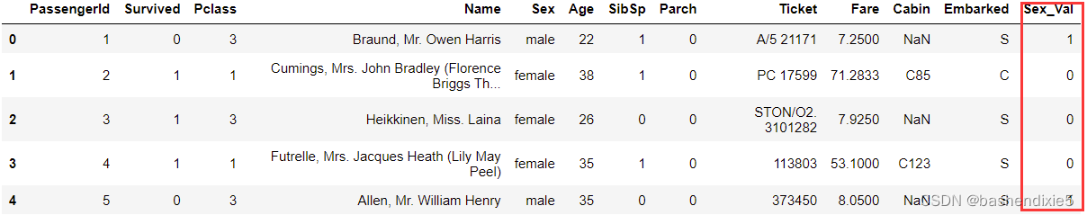
绘制 Sex_Val 和 Survived 的标准化交叉表:

大多数女性幸存下来,而大多数男性则没有。
接下来,我们将确定是否可以通过查看 Sex 和 Pclass 来获得有关存活率的任何见解。
计算每个 Pclass 中的男性和女性:
# Get the unique values of Pclass:
passenger_classes = sorted(df_train['Pclass'].unique())

for p_class in passenger_classes:
    print('M: ', p_class, len(df_train[(df_train['Sex'] == 'male') &
                             (df_train['Pclass'] == p_class)]))
    print('F: ', p_class, len(df_train[(df_train['Sex'] == 'female') &
                             (df_train['Pclass'] == p_class)]))
[5 rows x 13 columns]
M: 1 122
F: 1 94
M: 2 108
F: 2 76
M: 3 347
F: 3 144按性别和 Pclass 绘制生存率:
# Plot survival rate by Sex
females_df = df_train[df_train['Sex'] == 'female']
females_xt = pd.crosstab(females_df['Pclass'], df_train['Survived'])
females_xt_pct = females_xt.div(females_xt.sum(1).astype(float), axis=0)
females_xt_pct.plot(kind='bar',
                    stacked=True,
                    title='Female Survival Rate by Passenger Class')
plt.xlabel('Passenger Class')
plt.ylabel('Survival Rate')

# Plot survival rate by Pclass
males_df = df_train[df_train['Sex'] == 'male']
males_xt = pd.crosstab(males_df['Pclass'], df_train['Survived'])
males_xt_pct = males_xt.div(males_xt.sum(1).astype(float), axis=0)
males_xt_pct.plot(kind='bar',
                  stacked=True,
                  title='Male Survival Rate by Passenger Class')
plt.xlabel('Passenger Class')
plt.ylabel('Survival Rate')
plt.show()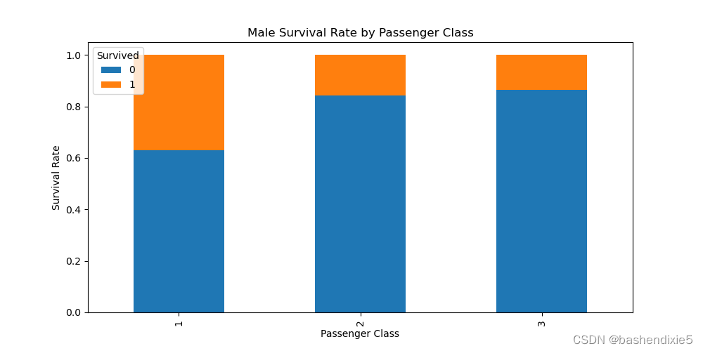
 一等和二等舱的绝大多数女性幸存下来。 头等舱的男性有最高的生存机会。
(9)特征:登船港口
Embarked 列可能是一个重要特征,但它缺少几个可能给机器学习算法带来问题的数据点:
df_train[df_train['Embarked'].isnull()]
准备将 Embarked 从字符串映射到数字表示:
# Get the unique values of Embarked
embarked_locs = df_train['Embarked'].unique()

embarked_locs_mapping = dict(zip(embarked_locs,
                                 range(0, len(embarked_locs) + 1)))
embarked_locs_mapping
{'S': 0, 'C': 1, 'Q': 2, nan: 3}将 Embarked 从字符串转换为数字表示:
df_train['Embarked_Val'] = df_train['Embarked'] \
                               .map(embarked_locs_mapping) \
                               .astype(int)
df_train.head()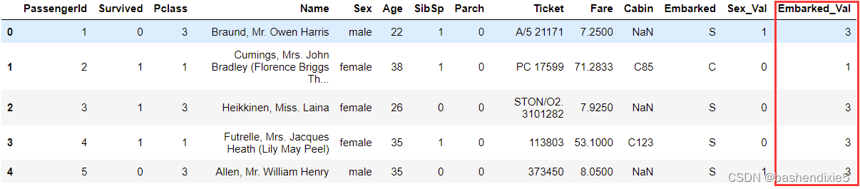
绘制 Embarked_Val 的直方图:
df_train['Embarked_Val'].hist(bins=len(embarked_locs), range=(0, 3))
plt.title('Port of Embarkation Histogram')
plt.xlabel('Port of Embarkation')
plt.ylabel('Count')
plt.show()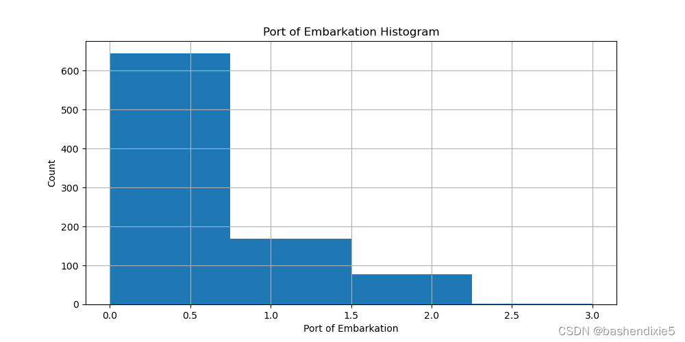
由于绝大多数乘客在 'S': 0 中登船,我们将 Embarked 中的缺失值分配给 'S':
for index in df_train['Embarked_Val'].index:
    if df_train['Embarked_Val'][index] ==3:
        df_train.loc[index] =0
然后检查一下
embarked_locs = sorted(df_train['Embarked_Val'].unique())
print(embarked_locs)
绘制 Embarked_Val 和 Survived 的标准化交叉表:
embarked_val_xt = pd.crosstab(df_train['Embarked_Val'], df_train['Survived'])
embarked_val_xt_pct = embarked_val_xt.div(embarked_val_xt.sum(1).astype(float), axis=0)
embarked_val_xt_pct.plot(kind='bar', stacked=True)
plt.title('Survival Rate by Port of Embarkation')
plt.xlabel('Port of Embarkation')
plt.ylabel('Survival Rate')
plt.show()
似乎那些在位置“C”:1 出发的人存活率最高。 我们将深入挖掘,看看为什么会出现这种情况。 下面我们绘制一个图表来确定每个港口的性别和乘客类别:
# Set up a grid of plots
fig = plt.figure(figsize=fizsize_with_subplots)

rows = 2
cols = 3
col_names = ('Sex_Val', 'Pclass')

for portIdx in embarked_locs:
    for colIdx in range(0, len(col_names)):
        plt.subplot2grid((rows, cols), (colIdx, portIdx))
        df_train[df_train['Embarked_Val'] == portIdx][col_names[colIdx]].value_counts().plot(kind='bar')

plt.show()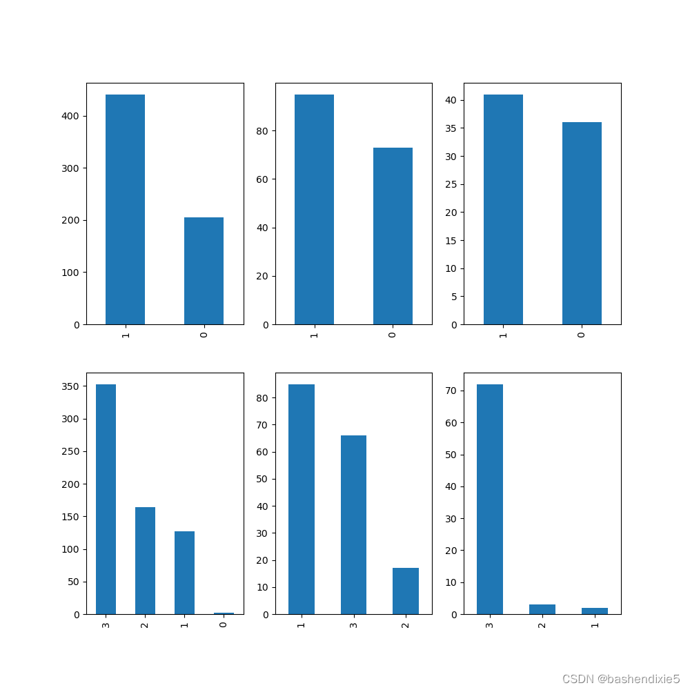
将 Embarked 保留为整数意味着对值进行排序,这并不存在。 另一种表示 Embarked 而不排序的方法是创建虚拟变量:
df_train = pd.concat([df_train, pd.get_dummies(df_train['Embarked_Val'], prefix='Embarked_Val')], axis=1)(10)特征:年龄
Age 列似乎是一个重要的特性——不幸的是它缺少许多值。 我们需要像使用 Embarked 一样填写缺失的值。
过滤以查看缺失的年龄值:
df_train[df_train['Age'].isnull()][['Sex', 'Pclass', 'Age']].head() 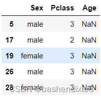
通过 Sex_Val 确定每个乘客类别的典型年龄。 我们将使用中位数而不是平均值,因为年龄直方图似乎是右偏斜的。
# To keep Age in tact, make a copy of it called AgeFill
# that we will use to fill in the missing ages:
df_train['AgeFill'] = df_train['Age']

# Populate AgeFill
df_train['AgeFill'] = df_train['AgeFill'] \
                        .groupby([df_train['Sex_Val'], df_train['Pclass']]) \
                        .apply(lambda x: x.fillna(x.median()))
确保 AgeFill 不包含任何缺失值:
len(df_train[df_train['AgeFill'].isnull()])绘制 AgeFill 和 Survived 的标准化交叉表:
# Set up a grid of plots
fig, axes = plt.subplots(2, 1, figsize=fizsize_with_subplots)

# Histogram of AgeFill segmented by Survived
df1 = df_train[df_train['Survived'] == 0]['Age']
df2 = df_train[df_train['Survived'] == 1]['Age']
max_age = max(df_train['AgeFill'])
axes[0].hist([df1, df2],
             bins=int(max_age / bin_size),
             range=(1, max_age),
             stacked=True)
axes[0].legend(('Died', 'Survived'), loc='best')
axes[0].set_title('Survivors by Age Groups Histogram')
axes[0].set_xlabel('Age')
axes[0].set_ylabel('Count')


# Scatter plot Survived and AgeFill
axes[1].scatter(df_train['Survived'], df_train['AgeFill'])
axes[1].set_title('Survivors by Age Plot')
axes[1].set_xlabel('Survived')
axes[1].set_ylabel('Age')
plt.show()
从上面的图表似乎没有清楚地显示任何规律。我们将继续深入挖掘。
按 Pclass 绘制 AgeFill 密度:
for pclass in passenger_classes:
    df_train.AgeFill[df_train.Pclass == pclass].plot(kind='kde')
plt.title('Age Density Plot by Passenger Class')
plt.xlabel('Age')
plt.legend(('1st Class', '2nd Class', '3rd Class'), loc='best')
plt.show()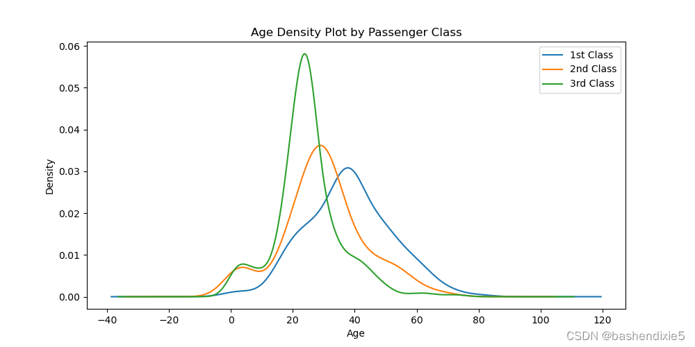
当按 Pclass 查看 AgeFill 密度时,我们看到头等舱乘客通常比二等舱乘客年龄大,而二等舱乘客又比三等舱乘客年龄大。 我们确定头等舱乘客的存活率高于二等舱乘客,而二等舱乘客的存活率又高于三等舱乘客。
# Set up a grid of plots
fig = plt.figure(figsize=fizsize_with_subplots)
fig_dims = (3, 1)

# Plot the AgeFill histogram for Survivors
plt.subplot2grid(fig_dims, (0, 0))
survived_df = df_train[df_train['Survived'] == 1]
survived_df['AgeFill'].hist(bins=int(max_age / bin_size), range=(1, max_age))

# Plot the AgeFill histogram for Females
plt.subplot2grid(fig_dims, (1, 0))
females_df = df_train[(df_train['Sex_Val'] == 0) & (df_train['Survived'] == 1)]
females_df['AgeFill'].hist(bins=int(max_age / bin_size), range=(1, max_age))

# Plot the AgeFill histogram for first class passengers
plt.subplot2grid(fig_dims, (2, 0))
class1_df = df_train[(df_train['Pclass'] == 1) & (df_train['Survived'] == 1)]
class1_df['AgeFill'].hist(bins=int(max_age / bin_size), range=(1, max_age))
plt.show()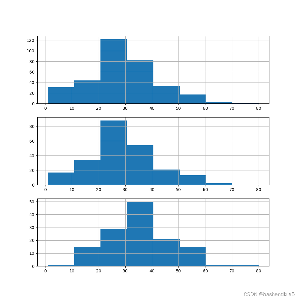
在第一张图中,我们看到大多数幸存者来自 20 到 30 岁的年龄段,可以通过以下两张图来解释。 第二张图显示大多数女性都在 20 多岁。 第三张图显示大多数头等舱乘客都在 30 多岁之内。
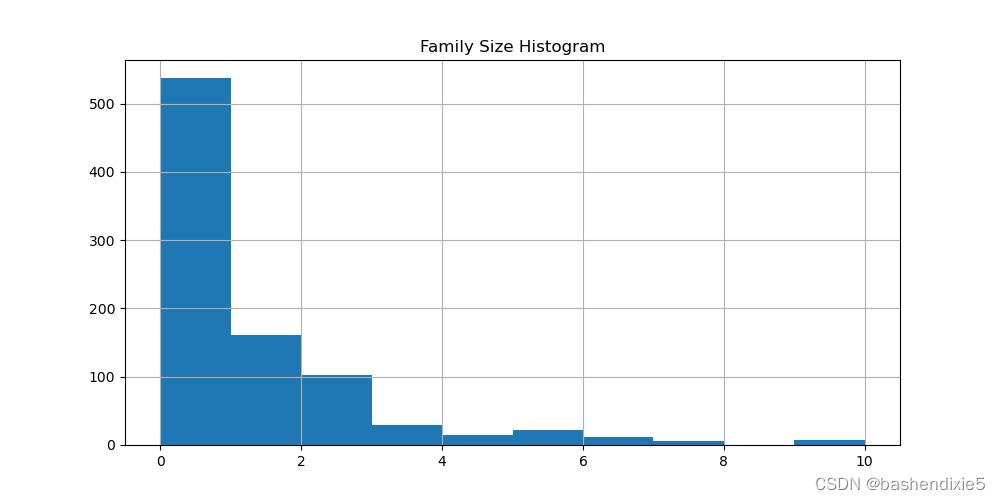
(11)特征:家庭规模
特征工程涉及创建新特征或修改可能对机器学习算法有利的现有特征。
定义一个新特征 FamilySize,它是 Parch(船上父母或孩子的数量)和 SibSp(兄弟姐妹或配偶的数量)之和:
df_train['FamilySize'] = df_train['SibSp'] + df_train['Parch']
df_train.head()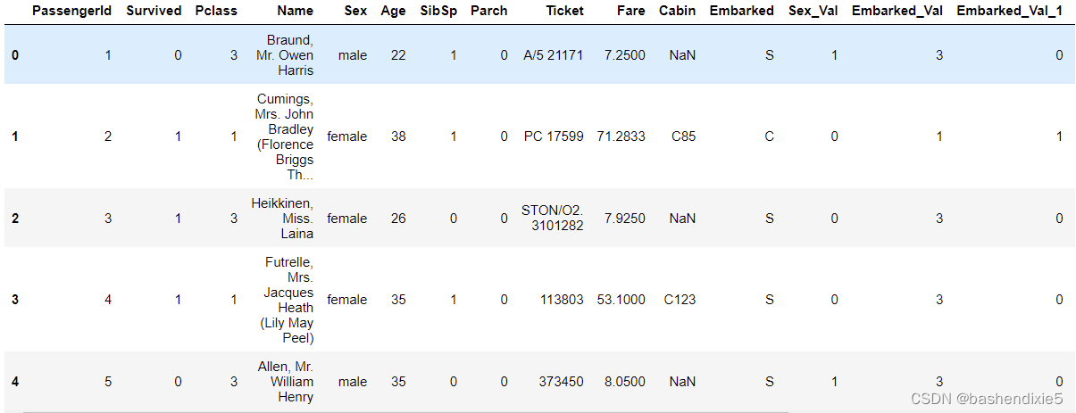
绘制 FamilySize 的直方图:
绘制由 Survived 分割的 AgeFill 直方图:
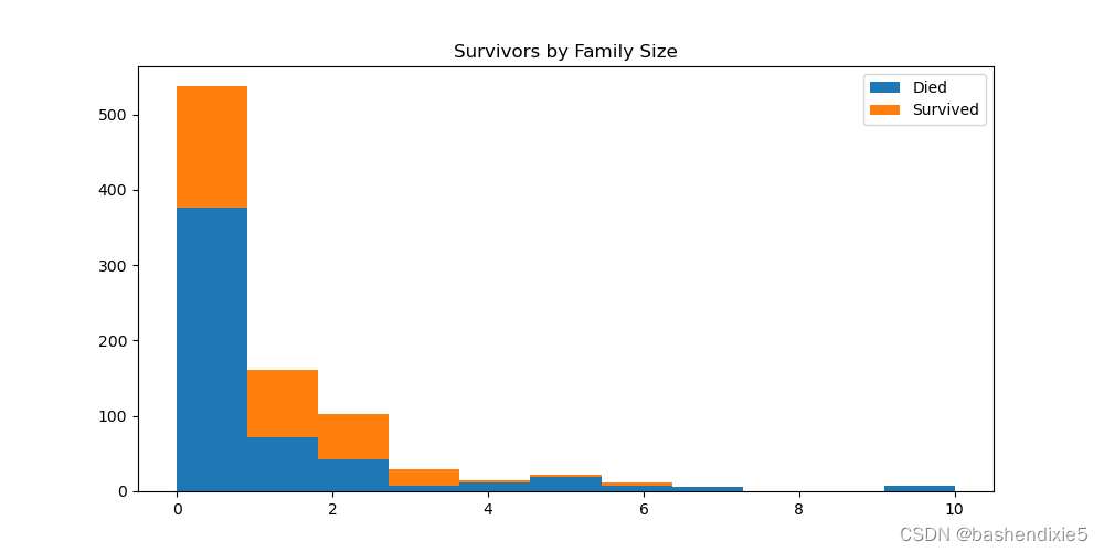
根据直方图,FamilySize 对生存的影响还不是很明显。不过机器学习算法也可能会从此功能中受益。
我们可能想要设计的其他功能可能与名称列相关,例如社会地位或头衔可能为男性的生存提供线索和更好的预测能力。
4、删除不需要的数据
许多机器学习算法不适用于字符串,它们通常要求数据位于数组中,而不是 DataFrame 中。
仅显示“对象”类型的列(字符串):
df_train.dtypes[df_train.dtypes.map(lambda x: x == 'object')]Name object
Sex object
Ticket object
Cabin object
Embarked object
dtype: object删除我们不会使用的列:
df_train = df_train.drop(['Name', 'Sex', 'Ticket', 'Cabin', 'Embarked'],
                         axis=1)
删除以下列:
Age 列,因为我们将使用 AgeFill 列。
SibSp 和 Parch 列,因为我们将使用 FamilySize 代替。
PassengerId 列,因为它不会用作特征。
Embarked_Val 因为我们决定使用虚拟变量。
df_train = df_train.drop(['Age', 'SibSp', 'Parch', 'PassengerId', 'Embarked_Val'], axis=1)
print(df_train.dtypes)
Survived int64
Pclass int64
Fare float64
Sex_Val int32
Embarked_Val_0 uint8
Embarked_Val_1 uint8
Embarked_Val_2 uint8
AgeFill float64
FamilySize int64
dtype: object将 DataFrame 转换为 numpy 数组:
[[ 0.      3.      7.25   ...  0.     22.      1.    ]
 [ 1.      1.     71.2833 ...  0.     38.      1.    ]
 [ 1.      3.      7.925  ...  0.     26.      0.    ]
 ...
 [ 0.      3.     23.45   ...  0.     21.5     3.    ]
 [ 1.      1.     30.     ...  0.     26.      0.    ]
 [ 0.      3.      7.75   ...  1.     32.      0.    ]]