通过示例学习Pytorch

简单理解梯度下降法

梯度下降（gradient descent）在机器学习中应用十分的广泛，不论是在线性回归还是Logistic回归中，它的主要目的是通过迭代找到目标函数的最小值，或者收敛到最小值。

梯度下降的基本过程就和下山的场景很类似。

首先，我们有一个可微分的函数。这个函数就代表着一座山。我们的目标就是找到这个函数的最小值，也就是山底。根据之前的场景假设，最快的下山的方式就是找到当前位置最陡峭的方向，然后沿着此方向向下走，对应到函数中，就是找到给定点的梯度 ，然后朝着梯度相反的方向，就能让函数值下降的最快！因为梯度的方向就是函数之变化最快的方向.
 

预热: NumPy

在介绍 PyTorch 之前，我们将首先使用 numpy 实现网络。

Numpy 提供了一个 n 维数组对象，以及许多用于操纵这些数组的函数。 Numpy 是用于科学计算的通用框架。 它对计算图，深度学习或梯度一无所知。 但是，通过使用 numpy 操作手动实现网络的前向和后向传递，我们可以轻松地使用 numpy 使三阶多项式适合正弦函数：

# -*- coding: utf-8 -*-
import numpy as np
import math

# Create random input and output data
x = np.linspace(-math.pi, math.pi, 2000)
y = np.sin(x)

# Randomly initialize weights
a = np.random.randn()
b = np.random.randn()
c = np.random.randn()
d = np.random.randn()

learning_rate = 1e-6
for t in range(2000):   # 随着迭代次数增加，损失值就会越小，但变化趋近于零
    # Forward pass: compute predicted y
    # y = a + b x + c x^2 + d x^3
    y_pred = a + b * x + c * x ** 2 + d * x ** 3

    # Compute and print loss
    # numpy.square（）函数返回一个新数组，该数组的元素值为源数组元素的平方，源阵列保持不变
    loss = np.square(y_pred - y).sum()
    if t % 100 == 99:
        print(t, loss)

    # Backprop to compute gradients of a, b, c, d with respect to loss
    # 反向传播来计算a, b, c, d关于损失的梯度
    grad_y_pred = 2.0 * (y_pred - y)
    grad_a = grad_y_pred.sum()
    grad_b = (grad_y_pred * x).sum()
    grad_c = (grad_y_pred * x ** 2).sum()
    grad_d = (grad_y_pred * x ** 3).sum()

    # Update weights
    a -= learning_rate * grad_a
    b -= learning_rate * grad_b
    c -= learning_rate * grad_c
    d -= learning_rate * grad_d

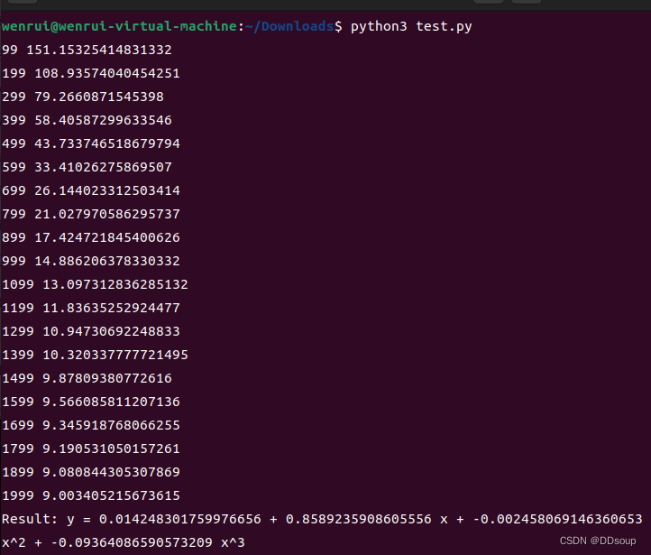
print(f'Result: y = {a} + {b} x + {c} x^2 + {d} x^3')

执行结果：

Pytorch ：张量

Numpy 是一个很棒的框架，但是它不能利用 GPU 来加速其数值计算。 对于现代深度神经网络，GPU 通常会提供 50 倍或更高的加速，因此遗憾的是，numpy 不足以实现现代深度学习。

在这里，我们介绍最基本的 PyTorch 概念：张量。 PyTorch 张量在概念上与 numpy 数组相同：张量是 n 维数组，PyTorch 提供了许多在这些张量上进行操作的函数。 在幕后，张量可以跟踪计算图和梯度，但它们也可用作科学计算的通用工具。

与 numpy 不同，PyTorch 张量可以利用 GPU 加速其数字计算。 要在 GPU 上运行 PyTorch 张量，您只需要指定正确的设备即可。

在这里，我们使用 PyTorch 张量将三阶多项式拟合为正弦函数。 像上面的 numpy 示例一样，我们需要手动实现通过网络的正向和反向传递：

# -*- coding: utf-8 -*-

import torch
import math

dtype = torch.float
device = torch.device("cpu")
# device = torch.device("cuda:0") # Uncomment this to run on GPU

# Create random input and output data
x = torch.linspace(-math.pi, math.pi, 2000, device=device, dtype=dtype)
y = torch.sin(x)

# Randomly initialize weights
a = torch.randn((), device=device, dtype=dtype)
b = torch.randn((), device=device, dtype=dtype)
c = torch.randn((), device=device, dtype=dtype)
d = torch.randn((), device=device, dtype=dtype)

learning_rate = 1e-6
for t in range(2000):
    # Forward pass: compute predicted y
    y_pred = a + b * x + c * x ** 2 + d * x ** 3

    # Compute and print loss
    loss = (y_pred - y).pow(2).sum().item()
    if t % 100 == 99:
        print(t, loss)

    # Backprop to compute gradients of a, b, c, d with respect to loss
    grad_y_pred = 2.0 * (y_pred - y)
    grad_a = grad_y_pred.sum()
    grad_b = (grad_y_pred * x).sum()
    grad_c = (grad_y_pred * x ** 2).sum()
    grad_d = (grad_y_pred * x ** 3).sum()

    # Update weights using gradient descent
    a -= learning_rate * grad_a
    b -= learning_rate * grad_b
    c -= learning_rate * grad_c
    d -= learning_rate * grad_d

print(f'Result: y = {a.item()} + {b.item()} x + {c.item()} x^2 + {d.item()} x^3')

张量与Autograd

        这里我们准备一个三阶多项式，通过最小化平方欧几里得距离来训练，并预测函数 y = sin(x) 在-pi到pi上的值。        

此实现使用了 PyTorch 张量(tensor)运算来实现前向传播，并使用 PyTorch Autograd 来计算梯度。

        PyTorch 张量表示计算图中的一个节点。 如果x是一个张量，且x.requires_grad=True，则x.grad是另一个张量，它保存了x相对于某个标量值的梯度。

import torch
import math

dtype = torch.float
device = torch.device("cpu")
# device = torch.device("cuda:0")  # Uncomment this to run on GPU

# Create Tensors to hold input and outputs.
# By default, requires_grad=False, which indicates that we do not need to
# compute gradients with respect to these Tensors during the backward pass.
x = torch.linspace(-math.pi, math.pi, 2000, device=device, dtype=dtype)
y = torch.sin(x)

# Create random Tensors for weights. For a third order polynomial, we need
# 4 weights: y = a + b x + c x^2 + d x^3
# Setting requires_grad=True indicates that we want to compute gradients with
# respect to these Tensors during the backward pass.
a = torch.randn((), device=device, dtype=dtype, requires_grad=True)
b = torch.randn((), device=device, dtype=dtype, requires_grad=True)
c = torch.randn((), device=device, dtype=dtype, requires_grad=True)
d = torch.randn((), device=device, dtype=dtype, requires_grad=True)

learning_rate = 1e-6
for t in range(2000):
    # Forward pass: compute predicted y using operations on Tensors.
    y_pred = a + b * x + c * x ** 2 + d * x ** 3

    # Compute and print loss using operations on Tensors.
    # Now loss is a Tensor of shape (1,)
    # loss.item() gets the scalar value held in the loss.
    loss = (y_pred - y).pow(2).sum()
    if t % 100 == 99:
        print(t, loss.item())

    # Use autograd to compute the backward pass. This call will compute the
    # gradient of loss with respect to all Tensors with requires_grad=True.
    # After this call a.grad, b.grad. c.grad and d.grad will be Tensors holding
    # the gradient of the loss with respect to a, b, c, d respectively.
    loss.backward()

    # Manually update weights using gradient descent. Wrap in torch.no_grad()
    # because weights have requires_grad=True, but we don't need to track this
    # in autograd.
    with torch.no_grad():
        a -= learning_rate * a.grad
        b -= learning_rate * b.grad
        c -= learning_rate * c.grad
        d -= learning_rate * d.grad

        # Manually zero the gradients after updating weights
        a.grad = None
        b.grad = None
        c.grad = None
        d.grad = None

print(f'Result: y = {a.item()} + {b.item()} x + {c.item()} x^2 + {d.item()} x^3')

使用torch.nn

        一个三阶多项式，通过最小化平方欧几里得距离来训练，并预测函数 y = sin(x) 在-pi到pi上的值。

        这个实现使用 PyTorch 的nn包来构建神经网络。 PyTorch Autograd 让我们定义计算图和计算梯度变得容易了，但是原始的 Autograd 对于定义复杂的神经网络来说可能太底层了。 这时候nn包就能帮上忙。 nn包定义了一组模块，你可以把它视作一层神经网络，该神经网络层接受输入，产生输出，并且可能有一些可训练的权重。

import torch
import math

# Create Tensors to hold input and outputs
x = torch.linspace(-math.pi,math.pi,2000)
y = torch.sin(x)

# tensor (x, x^2, x^3)
p = torch.tensor([1,2,3])
xx = x.unsqueeze(-1).pow(p)

model = torch.nn.Sequential(
    torch.nn.Linear(3,1),
    torch.nn.Flatten(0,1)
)

loss_fn = torch.nn.MSELoss(reduction='sum')

learning_rate = 1e-6
for t in range(2000):
    y_pred = model(xx)
    loss = loss_fn(y_pred,y)
    if t%100==99:
        print(t,loss.item())

    model.zero_grad()

    loss.backward()

    with torch.no_grad():
        for param in model.parameters():
            param -= learning_rate * param.grad

linear_layer = model[0]
print(f'Result: y = {linear_layer.bias.item()} + {linear_layer.weight[:, 0].item()} x + {linear_layer.weight[:, 1].item()} x^2 + {linear_layer.weight[:, 2].item()} x^3')

使用 optim

        延续上面的例子：

        与其像以前那样手动更新模型的权重，不如使用optim包定义一个优化器，该优化器将为我们更新权重。 optim包定义了许多深度学习常用的优化算法，包括 SGD + 动量，RMSProp，Adam 等。

import torch
import math

# Create Tensors to hold input and outputs
x = torch.linspace(-math.pi,math.pi,2000)
y = torch.sin(x)

# tensor (x, x^2, x^3)
p = torch.tensor([1,2,3])
xx = x.unsqueeze(-1).pow(p)

model = torch.nn.Sequential(
    torch.nn.Linear(3,1),
    torch.nn.Flatten(0,1)
)

loss_fn = torch.nn.MSELoss(reduction='sum')

learning_rate = 1e-3
optimizer = torch.optim.RMSprop(model.parameters(), lr=learning_rate)
for t in range(2000):
    y_pred = model(xx)
    loss = loss_fn(y_pred,y)
    if t%100==99:
        print(t,loss.item())

    optimizer.zero_grad()

    loss.backward()

    optimizer.step()

linear_layer = model[0]
print(f'Result: y = {linear_layer.bias.item()} + {linear_layer.weight[:, 0].item()} x + {linear_layer.weight[:, 1].item()} x^2 + {linear_layer.weight[:, 2].item()} x^3')

自定义nn模块

        此实现将模型定义为自定义Module子类。想要一个比现有模块的简单序列更复杂的模型时，都需要以这种方式定义模型。

import torch
import math

class SZTU(torch.nn.Module):
    def __init__(self):
        super().__init__()
        self.a = torch.nn.Parameter(torch.randn(()))
        self.b = torch.nn.Parameter(torch.randn(()))
        self.c = torch.nn.Parameter(torch.randn(()))
        self.d = torch.nn.Parameter(torch.randn(()))

    def forward(self, x):
        return self.a + self.b * x + self.c * x ** 2 + self.d * x ** 3

    def string(self):
        return f'y = {self.a.item()} + {self.b.item()} x + {self.c.item()} x^2 + {self.d.item()} x^3'

x = torch.linspace(-math.pi, math.pi, 2000)
y = torch.sin(x)

model = SZTU()

criterion = torch.nn.MSELoss(reduction='sum')
optimizer = torch.optim.SGD(model.parameters(), lr = 1e-6)

for t in range(2000):
    y_pred = model(x)

    loss = criterion(y_pred, y)
    if t % 100 == 99:
        print(t, loss.item())

    optimizer.zero_grad()
    loss.backward()
    optimizer.step()

print(f'Result: {model.string()}')