基于BP神经网络对MNIST数据集检测识别（numpy版本）

1．作者介绍

王凯，男，西安工程大学电子信息学院，2022级研究生
研究方向：机器视觉与人工智能
电子邮件：[email protected]

张思怡，女，西安工程大学电子信息学院，2022级研究生，张宏伟人工智能课题组
研究方向：机器视觉与人工智能
电子邮件：[email protected]

2．BP神经网络介绍

2.1 BP神经网络

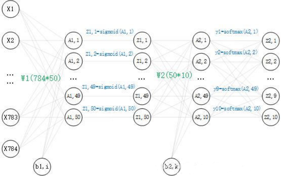
搭建一个两层（两个权重矩阵，一个隐藏层）的神经网络，其中输入节点和输出节点的个数是确定的，分别为 784 和 10。而隐藏层节点的个数还未确定，并没有明确要求隐藏层的节点个数，所以在这里取50个。现在神经网络的结构已经确定了，再看一下里面是怎么样的，这里画出了对一个数据的运算过程：

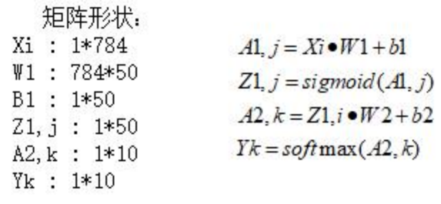
数学公式：

3．BP神经网络对MNIST数据集检测实验

3.1 读取数据集

安装numpy :pip install numpy
安装matplotlib pip install matplotlib
mnist是一个包含各种手写数字图片的数据集：其中有60000个训练数据和10000个测试时局，即60000个 train_img 和与之对应的 train_label，10000个 test_img 和 与之对应的test_label。

其中的 train_img 和 test_img 就是这种图片的形式，train_img 是为了训练神经网络算法的训练数据，test_img 是为了测试神经网络算法的测试数据，每一张图片为2828，将图片转换为2828=784个像素点，每个像素点的值为0到255，像素点值的大小代表灰度，从而构成一个1784的矩阵，作为神经网络的输入，而神经网络的输出形式为110的矩阵，个：eg：[0.01，0.01，0.01，0.04，0.8，0.01，0.1，0.01，0.01，0.01]，矩阵里的数字代表神经网络预测值的概率，比如0.8代表第五个数的预测值概率。
其中 train_label 和 test_label 是 对应训练数据和测试数据的标签，可以理解为一个1*10的矩阵，用one-hot-vectors（只有正确解表示为1）表示，one_hot_label为True的情况下，标签作为one-hot数组返回，one-hot数组 例：[0，0，0，0，1，0，0，0，0，0]，即矩阵里的数字1代表第五个数为True，也就是这个标签代表数字5。
数据集的读取：
load_mnist(normalize=True, flatten=True, one_hot_label=False):中，
normalize : 是否将图像的像素值正规化为0.0~1.0（将像素值正规化有利于提高精度）。flatten : 是否将图像展开为一维数组。 one_hot_label:是否采用one-hot表示。

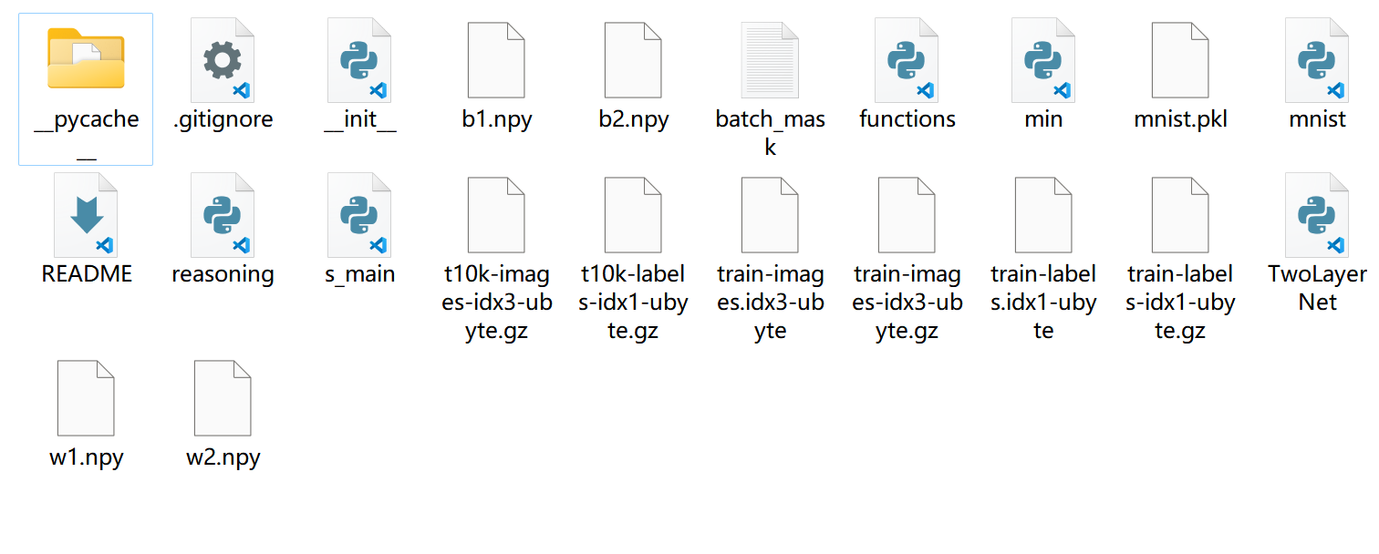
完整代码及数据集下载：https://gitee.com/wang-kai-ya/bp.git

3.2 前向传播

前向传播时，我们可以构造一个函数，输入数据，输出预测。

def predict(self, x):
    w1, w2 = self.dict['w1'], self.dict['w2']
    b1, b2 = self.dict['b1'], self.dict['b2']

    a1 = np.dot(x, w1) + b1
    z1 = sigmoid(a1)
    a2 = np.dot(z1, w2) + b2
    y = softmax(a2)

3.3 损失函数

求出神经网络对一组数据的预测值，是一个1*10的矩阵。

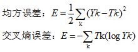
其中，Yk表示的是第k个节点的预测值，Tk表示标签中第k个节点的one-hot值，举前面的eg：（手写数字5的图片预测值和5的标签）
Yk=[0.01，0.01，0.01，0.04，0.8，0.01，0.1，0.01，0.01，0.01]
Tk=[0, 0, 0, 0, 1, 0, 0, 0, 0, 0]
值得一提的是，在交叉熵误差函数中，Tk的值只有一个1，其余为0，所以对于这个数据的交叉熵误差就为 E = -1（log0.8）。
在这里选用交叉熵误差作为损失函数，代码实现如下：

def loss(self, y, t):
    t = t.argmax(axis=1)
    num = y.shape[0]
    s = y[np.arange(num), t]

    return -np.sum(np.log(s)) / num

3.4 构建神经网络

前面我们定义了预测值predict, 损失函数loss, 识别精度accuracy, 梯度grad，下面构建一个神经网络的类，把这些方法添加到神经网络的类中：

for i in range(epoch):
    batch_mask = np.random.choice(train_size, batch_size)  # 从0到60000 随机选100个数
    x_batch = x_train[batch_mask]
    y_batch = net.predict(x_batch)
    t_batch = t_train[batch_mask]
    grad = net.gradient(x_batch, t_batch)

    for key in ('w1', 'b1', 'w2', 'b2'):
        net.dict[key] -= lr * grad[key]
    loss = net.loss(y_batch, t_batch)
    train_loss_list.append(loss)

    # 每批数据记录一次精度和当前的损失值
    if i % iter_per_epoch == 0:
        train_acc = net.accuracy(x_train, t_train)
        test_acc = net.accuracy(x_test, t_test)
        train_acc_list.append(train_acc)
        test_acc_list.append(test_acc)
        print(
            '第' + str(i/600) + '次迭代''train_acc, test_acc, loss :| ' + str(train_acc) + ", " + str(test_acc) + ',' + str(
                loss))

3.5 训练

import numpy as np
import matplotlib.pyplot as plt
from TwoLayerNet import TwoLayerNet
from mnist import load_mnist

(x_train, t_train), (x_test, t_test) = load_mnist(normalize=True, one_hot_label=True)
net = TwoLayerNet(input_size=784, hidden_size=50, output_size=10, weight_init_std=0.01)

epoch = 20400
batch_size = 100
lr = 0.1

train_size = x_train.shape[0]  # 60000
iter_per_epoch = max(train_size / batch_size, 1)  # 600

train_loss_list = []
train_acc_list = []
test_acc_list = []

保存权重：

np.save('w1.npy', net.dict['w1'])
np.save('b1.npy', net.dict['b1'])
np.save('w2.npy', net.dict['w2'])
np.save('b2.npy', net.dict['b2'])

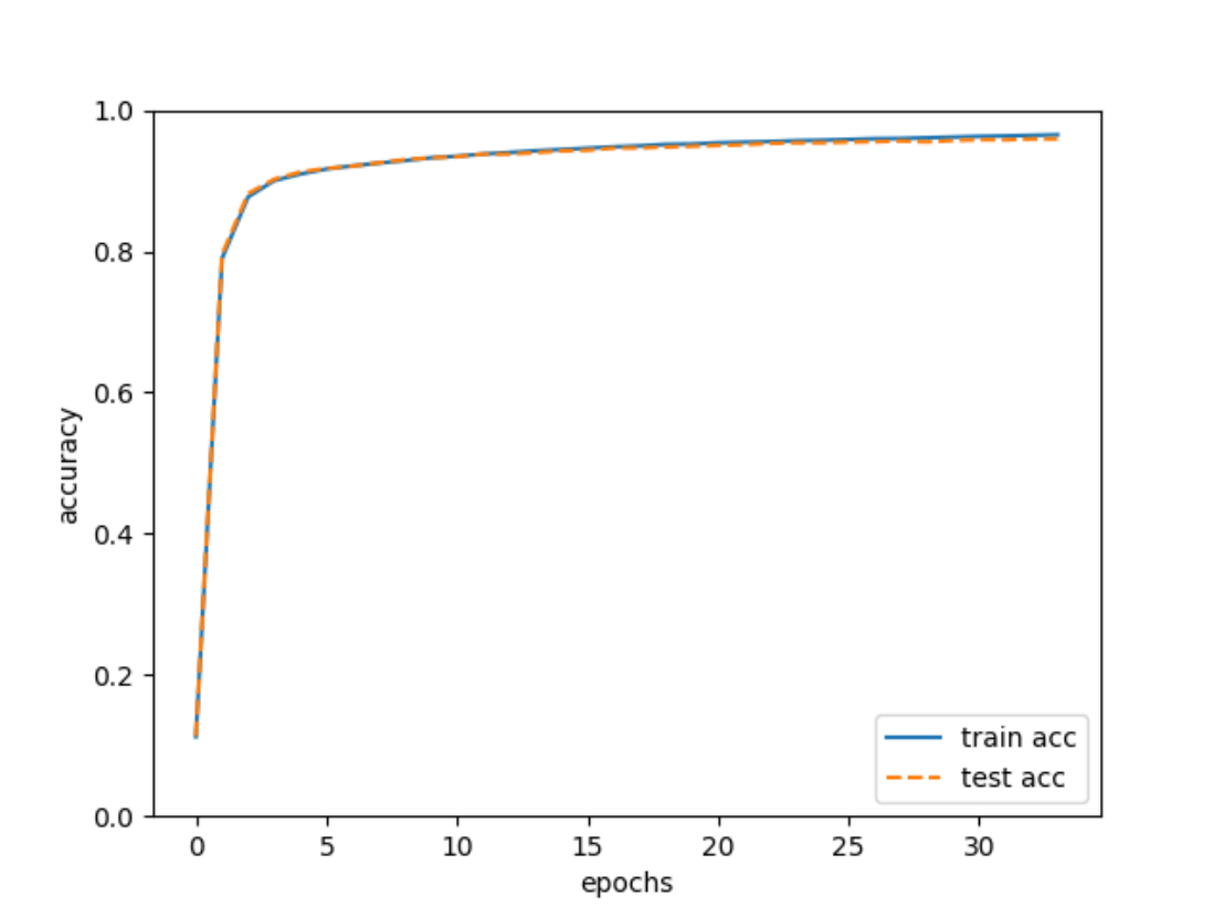
结果可视化：

3.6 模型推理

import numpy as np
from mnist import load_mnist
from functions import sigmoid, softmax
import cv2
######################################数据的预处理
(x_train, t_train), (x_test, t_test) = load_mnist(normalize=True, one_hot_label=True)
batch_mask = np.random.choice(100,1)  # 从0到60000 随机选100个数
#print(batch_mask)
x_batch = x_train[batch_mask]

#####################################转成图片
arr = x_batch.reshape(28,28)
cv2.imshow('wk',arr)
key = cv2.waitKey(10000)
#np.savetxt('batch_mask.txt',arr)
#print(x_batch)
#train_size = x_batch.shape[0]
#print(train_size)
########################################进入模型预测
w1 = np.load('w1.npy')
b1 = np.load('b1.npy')
w2 = np.load('w2.npy')
b2 = np.load('b2.npy')

a1 = np.dot(x_batch,w1) + b1
z1 = sigmoid(a1)
a2 = np.dot(z1,w2) + b2
y = softmax(a2)
p = np.argmax(y, axis=1)

print(p)

运行python reasoning.py
可以看到模型拥有较高的准确率。

4．完整代码

训练

import numpy as np
import matplotlib.pyplot as plt
from TwoLayerNet import TwoLayerNet
from mnist import load_mnist

(x_train, t_train), (x_test, t_test) = load_mnist(normalize=True, one_hot_label=True)
net = TwoLayerNet(input_size=784, hidden_size=50, output_size=10, weight_init_std=0.01)

epoch = 20400
batch_size = 100
lr = 0.1

train_size = x_train.shape[0]  # 60000
iter_per_epoch = max(train_size / batch_size, 1)  # 600

train_loss_list = []
train_acc_list = []
test_acc_list = []

for i in range(epoch):
    batch_mask = np.random.choice(train_size, batch_size)  # 从0到60000 随机选100个数
    x_batch = x_train[batch_mask]
    y_batch = net.predict(x_batch)
    t_batch = t_train[batch_mask]
    grad = net.gradient(x_batch, t_batch)

    for key in ('w1', 'b1', 'w2', 'b2'):
        net.dict[key] -= lr * grad[key]
    loss = net.loss(y_batch, t_batch)
    train_loss_list.append(loss)

    # 每批数据记录一次精度和当前的损失值
    if i % iter_per_epoch == 0:
        train_acc = net.accuracy(x_train, t_train)
        test_acc = net.accuracy(x_test, t_test)
        train_acc_list.append(train_acc)
        test_acc_list.append(test_acc)
        print(
            '第' + str(i/600) + '次迭代''train_acc, test_acc, loss :| ' + str(train_acc) + ", " + str(test_acc) + ',' + str(
                loss))

np.save('w1.npy', net.dict['w1'])
np.save('b1.npy', net.dict['b1'])
np.save('w2.npy', net.dict['w2'])
np.save('b2.npy', net.dict['b2'])

markers = {'train': 'o', 'test': 's'}
x = np.arange(len(train_acc_list))
plt.plot(x, train_acc_list, label='train acc')
plt.plot(x, test_acc_list, label='test acc', linestyle='--')
plt.xlabel("epochs")
plt.ylabel("accuracy")
plt.ylim(0, 1.0)
plt.legend(loc='lower right')
plt.show()

测试

import numpy as np
from mnist import load_mnist
from functions import sigmoid, softmax
import cv2
######################################数据的预处理
(x_train, t_train), (x_test, t_test) = load_mnist(normalize=True, one_hot_label=True)
batch_mask = np.random.choice(100,1)  # 从0到60000 随机选100个数
#print(batch_mask)
x_batch = x_train[batch_mask]

#####################################转成图片
arr = x_batch.reshape(28,28)
cv2.imshow('wk',arr)
key = cv2.waitKey(10000)
#np.savetxt('batch_mask.txt',arr)
#print(x_batch)
#train_size = x_batch.shape[0]
#print(train_size)
########################################进入模型预测
w1 = np.load('w1.npy')
b1 = np.load('b1.npy')
w2 = np.load('w2.npy')
b2 = np.load('b2.npy')

a1 = np.dot(x_batch,w1) + b1
z1 = sigmoid(a1)
a2 = np.dot(z1,w2) + b2
y = softmax(a2)
p = np.argmax(y, axis=1)

print(p)