tensorflow卷积神经网络识别mnist数据集

tensorflow卷积神经网络识别mnist数据集

在之前我使用过简单的神经网络来识别mnist手写数据，但是效果并不是很好，因为简单的神经网络在隐层里面只有一层就是全连接层，神经网络并不复杂所以导致识别正确率只有93%左右。而卷积神经网络在图像识别方面是做得比较好的，卷积神经网络经过不断地优化和发展，它除了可以简单的识别图像，也可以描绘图像和识别比较复杂的图像。

观察mnist图片

在我们读取数据的时候是无法看到图片的样子，所以在建立模型之前先读出图片观察一下图片内容

import tensorflow as tf
from tensorflow.examples.tutorials.mnist import input_data
import matplotlib.pyplot as plt
mnist = input_data.read_data_sets(r"I:\crack\DATA\数字", one_hot=True)

img = mnist.train.images[13]
label = mnist.train.labels[13]

plt.figure()


plt.subplot(2,2,3)
plt.imshow(img.reshape(28,28),cmap='gray')
plt.axis('off')

plt.show()

with tf.Session() as sess:
    print(label)

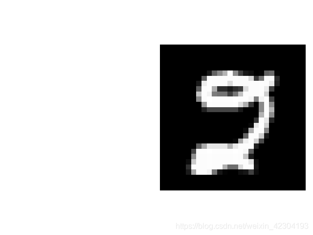
这里我只是提取了一个图片来观察的，这个图片类别是2，也就代表了这个图片的信息是数字2，但是不太符合我写数字的习惯。

卷积神经网络的结构

在tensorflow里面识别mnist手写数字在隐层里面用了三层结构，而经过我的实验，在隐层里面只要有两层卷积层效果就已经足够好了。

这次的卷积神经网络的结构有5层：输入层、第一层卷积层、第二层卷积层、全连接层、输出层。

输入层

from tensorflow.examples.tutorials.mnist import input_data
mnist = input_data.read_data_sets(r"I:\crack\DATA\数字",one_hot=True)
#读取数据
with tf.variable_scope("data"):
    #建立占位符，首先是输入图片数据的占位符
    x = tf.placeholder(tf.float32, shape=[None, 784], name="x_data")
    y_ture = tf.placeholder(tf.float32, shape=[None, 10], name="y_data")

在这里为了让在网页上面呈现的图片更加清楚，所以用区域块来包裹着每一部分。
然后先用占位符先提前占一个位置方面后面再输入数据。
因为mnist数据集已经被加密过了，所以要用特殊的方式来读取。

第一层卷积层

#第一层卷积层,fillter数量为32，扫描框大小为5*5，通道数为1，步长为1
with tf.variable_scope("convolution_1"):
    #随机生成权重和偏执
    weight_1 = tf.Variable(tf.random_normal(shape=[5,5,1,32],stddev=0.1),name="weight_1")
    bias_1 = tf.Variable(tf.constant(0.1,shape=[32]), name="bias_1")
    x_data = tf.reshape(x,shape=[-1,28,28,1])
    #卷积计算和激活函数和池化计算
    relu_1 = tf.nn.relu(tf.nn.conv2d(x_data,weight_1,strides=[1,1,1,1],padding="SAME") + bias_1)
    pool_1 = tf.nn.max_pool(relu_1,ksize=[1,2,2,1],strides=[1,2,2,1],padding="SAME")

首先卷积计算的流程是这样的：就是定义一个过滤器，就是定义一个扫描框，然后扫描框定义在图片一个地方，然后扫描这个框里面图片的像素值然后进行线性回归的计算得出一个值，然后扫描框再向下移，然后再用线性回归计算出一个值，相当于这个扫描框在把这张图片进行扫描得出多个计算的值。扫描框的大小一般都是奇数乘于奇数的大小。这里的扫描器可以是多个，然后得出多个表结构的结果。

因为卷积计算涉及的是线性回归的计算，所以也需要权重和偏执，这样的权重和偏执的设置要小心，因为我验证过了，不是任意随机生成的，随机生成的权重的标准差要是0.1或者是0.0，因为过大会导致模型调整不过来。

第二层卷积层

第二层卷积层
with tf.variable_scope("convolution_2"):
    weight_2 = tf.Variable(tf.random_normal(shape=[5,5,32,64],stddev=0.1),name="weight_2")
    bias_2 = tf.Variable(tf.constant(1.0,shape=[64]), name="bias_2")
    relu_2 = tf.nn.relu(tf.nn.conv2d(pool_1,weight_2,strides=[1,1,1,1],padding="SAME") + bias_2)
    pool_2 = tf.nn.max_pool(relu_2,ksize=[1,2,2,1],strides=[1,2,2,1],padding="SAME")
    #删除一部分值，防止过拟合
    data_drop = tf.nn.dropout(pool_2,keep_prob=0.4)

第二层卷积层的fillter是64，宽度还是5 * 5，步长还是1，因为这里的输入值是上面输出的值，所以通道数就变成了32

这里删除了数据的百分之四十的值，就是为了模型过拟合

全连接层

#全连接层
with tf.variable_scope("model"):
    weight = tf.Variable(tf.random_normal(shape=[7*7*64, 10],stddev=0.1),name="weight")
    bias = tf.Variable(tf.constant(0.1,shape=[10]), name="bias")
    data = tf.reshape(data_drop,[-1,7*7*64])
    predict = tf.matmul(data, weight) + bias

这里因为上面输出的数据形状是[None,7,7,64]，所以要动态修改一下形状，然后用矩阵相乘的方式得出结果。

得出预测的值并计算交叉熵平均损失

#然后开始用softmax预测出结果和交叉熵的计算
with tf.variable_scope("soft_croos"):
    #计算出交叉熵损失的列表
    y_conv = tf.nn.softmax(predict)
    # 然后计算出平均值
    cross_entropy = -tf.reduce_sum(y_ture * tf.log(y_conv))

这里交叉熵损失计算也可以借鉴我上一篇博客的计算方式计算，得出的结果是一样的

梯度下降模型优化

with tf.variable_scope("optimize"):
    train_step = tf.train.AdamOptimizer(0.0001).minimize(cross_entropy)

计算准确率

with tf.variable_scope("accuracy"):
    correct_predict = tf.equal(tf.argmax(y_conv, 1), tf.argmax(y_ture, 1))
    accuracy = tf.reduce_mean(tf.cast(correct_predict, dtype=tf.float32))

初始化变量

#初始化op
init_op = tf.global_variables_initializer()

这里的初始化变量是一定要加的，如果图里面有变量而不加初始化变量这个功能的话就会报错

保存模型

#保存模型
saver = tf.train.Saver({“weight_1”:weight_1,"weight_2":weight_2,"weight":weight,"bias_1":bias_1,"bias_2":bias_2,"bias":bias})
saver.save(sess, r"I:\crack\ckpt-model2\model")

在建立保存模型的对象时一定要传递参数，不然在保存好的模型里面找不到这些参数

开启会话运行

with tf.Session() as sess:
    #初始化op
    sess.run(init_op)
    n = 1
    #随机拿出100个样本来训练，训练2000次
    for i in range(200):
        batch = mnist.train.next_batch(100)
        # 在相同100个样本中训练优化100次
        for j in range(100):
            # 每100次输出一次日志
            sess.run(train_step,feed_dict={x: batch[0], y_ture: batch[1]})
            print("训练步数{0}, 准确率：{1}".format(n, sess.run(accuracy, feed_dict={x: batch[0], y_ture: batch[1]})))
            n = n + 1
    #训练完成之后就保存模型
    saver.save(sess, r"I:\crack\ckpt-model2\model")

这里的训练模型的流程是，先循环200次，每次拿100个样本出来训练，然后循环优化100次，最后训练完了就保存模型。

使用测试集测试准确率

#然后加载模型，查看训练效果
    saver.restore(sess,r"I:\crack\ckpt-model2\model")
    image_batch = mnist.test.next_batch(1000)
    print("*"*1000)
    print(sess.run(accuracy, feed_dict={x: image_batch[0], y_ture: image_batch[1]}))

这里测试集得出来的准确率为0.959，因为这里的训练步数不是很多，但是相对于简单的神经网络的正确率已经高出很多了。

源代码

'''
卷积神经网络的手写数字识别
creat on September 7,2019
@Author 小明
'''
import tensorflow as tf
import numpy as np

'''
步骤：
1、读取数据
2、建立两层大型的卷积层
3、建立神经网络模型
4、预测结果和计算交叉熵
5、优化模型
6、保存模型和可视化观察模型
'''
from tensorflow.examples.tutorials.mnist import input_data
mnist = input_data.read_data_sets(r"I:\crack\DATA\数字",one_hot=True)


#读取数据
with tf.variable_scope("data"):
    #建立占位符，首先是输入图片数据的占位符
    x = tf.placeholder(tf.float32, shape=[None, 784], name="x_data")
    y_ture = tf.placeholder(tf.float32, shape=[None, 10], name="y_data")

#第一层卷积层,fillter数量为32，扫描框大小为5*5，通道数为1，步长为1
with tf.variable_scope("convolution_1"):
    #随机生成权重和偏执
    weight_1 = tf.Variable(tf.random_normal(shape=[5,5,1,32],stddev=0.1),name="weight_1")
    bias_1 = tf.Variable(tf.constant(0.1,shape=[32]), name="bias_1")
    x_data = tf.reshape(x,shape=[-1,28,28,1])
    #卷积计算和激活函数和池化计算
    relu_1 = tf.nn.relu(tf.nn.conv2d(x_data,weight_1,strides=[1,1,1,1],padding="SAME") + bias_1)
    pool_1 = tf.nn.max_pool(relu_1,ksize=[1,2,2,1],strides=[1,2,2,1],padding="SAME")

#第二层卷积层
with tf.variable_scope("convolution_2"):
    weight_2 = tf.Variable(tf.random_normal(shape=[5,5,32,64],stddev=0.1),name="weight_2")
    bias_2 = tf.Variable(tf.constant(1.0,shape=[64]), name="bias_2")
    relu_2 = tf.nn.relu(tf.nn.conv2d(pool_1,weight_2,strides=[1,1,1,1],padding="SAME") + bias_2)
    pool_2 = tf.nn.max_pool(relu_2,ksize=[1,2,2,1],strides=[1,2,2,1],padding="SAME")

#删除一部分的值，避免过拟合
    data_drop = tf.nn.dropout(pool_2,keep_prob=0.4)

#全连接层
with tf.variable_scope("model"):
    weight = tf.Variable(tf.random_normal(shape=[7*7*64, 10],stddev=0.1),name="weight")
    bias = tf.Variable(tf.constant(0.1,shape=[10]), name="bias")
    data = tf.reshape(data_drop,[-1,7*7*64])
    predict = tf.matmul(data, weight) + bias

#然后开始用softmax预测出结果和交叉熵的计算
with tf.variable_scope("soft_croos"):
    #计算出交叉熵损失的列表
    y_conv = tf.nn.softmax(predict)
    # 然后计算出平均值
    cross_entropy = -tf.reduce_sum(y_ture * tf.log(y_conv))

#求出梯度下降的损失，并且也是优化
with tf.variable_scope("optimize"):
    train_step = tf.train.AdamOptimizer(0.0001).minimize(cross_entropy)

#计算准确率
with tf.variable_scope("accuracy"):
    correct_predict = tf.equal(tf.argmax(y_conv, 1), tf.argmax(y_ture, 1))
    accuracy = tf.reduce_mean(tf.cast(correct_predict, dtype=tf.float32))

#初始化op
init_op = tf.global_variables_initializer()

#保存模型
saver = tf.train.Saver()

with tf.Session() as sess:
    #初始化op
    sess.run(init_op)
    n = 1
    #随机拿出100个样本来训练，训练2000次
    for i in range(200):
        batch = mnist.train.next_batch(100)
        # 在相同100个样本中训练优化100次
        for j in range(100):
            # 每100次输出一次日志
            sess.run(train_step,feed_dict={x: batch[0], y_ture: batch[1]})
            print("训练步数{0}, 准确率：{1}".format(n, sess.run(accuracy, feed_dict={x: batch[0], y_ture: batch[1]})))
            n = n + 1
    #训练完成之后就保存模型
    saver.save(sess, r"I:\crack\ckpt-model2\model")

    #然后加载模型，查看训练效果
    saver.restore(sess,r"I:\crack\ckpt-model2\model")
    image_batch = mnist.test.next_batch(1000)
    print("*"*1000)
    print(sess.run(accuracy, feed_dict={x: image_batch[0], y_ture: image_batch[1]}))

如果对上面代码有什么疑惑的，可以添加我的QQ 1693490575，我们一起来探讨！