1、数据解释
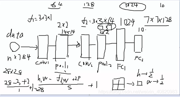
两个卷积层,池化层,全连接层。数量关系见下图。
输入格式:28*28*1 55000张(程序中只选了一部分)
conv1:filter1 =3*3*1 , pad=1 ,stride=1
输出特征图:28*28*64 计算公式: =28,宽w同理。
池化层: pool1:2*2 输出:14*14*64
conv2: filter2=3*3*64 , pad=1 stride=1
输出特征图:14*14*128
池化层: pool2:2*2 输出:7*7*128
全连接层:fc1 : [7*7*128,1024 ] fc2:[1024,10]

2、函数介绍
(1)tf.nn.conv2d(input, filter, strides, padding)
输入格式[batch, in_height, in_width, in_channels]
卷积核[filter_height, filter_width, in_channels, out_channels]
stride: [1,h,w,1]
padding: A `string` from: `"SAME", "VALID"`.
(2)tf.shape()获取张量的大小,返回tensor类型。array 、list、 tensor 类型都可以用,可用sess.run(tf.shape())获得array类型输出。例如: sess.run(tf.shape(array))
tf.get_shape() 获取大小,只有tensor类型可用,返回元组,需用as_list()转换为list类型。不需要用sess.run()。 例如:tf.get_shape().as_list(tensor_variable)
tf.reshape(tensor_variable, [x,y,z] )或 [x,y] , 若有一维不确定,可以用-1 代替,系统根据原变量的大小和已知参数计算。
(3)见https://blog.csdn.net/mieleizhi0522/article/details/80416668
tf.nn.bias_add():
一个叫bias的向量加到一个叫value的矩阵上,是向量与矩阵的每行(或每维)进行相加,得到的结果和value矩阵大小相同。
官方解释:
bias: A 1-D `Tensor` with size matching the last dimension of `value`.
tf.add( x,y, name=None):
这个情况比较多,最常见的是,一个叫x的矩阵和一个叫y的数相加,就是y分别与x的每个数相加,得到的结果和x大小相同。
tf.add_n(inputs,name=None)
实现一个列表的元素的相加。就是输入的对象是一个列表,列表里的元素可以是向量,矩阵等但没有广播功能
(4)
optm = tf.train.AdamOptimizer(learning_rate=0.001).minimize(cost) 优化函数,详见:https://blog.csdn.net/shenxiaoming77/article/details/77169756
完整代码:
#!/usr/bin/env python
# -*- coding:utf-8 -*-
#@Time  : 2018/12/11 17:29
#@Author: little bear
#@File  : tf_mnistCNN.py

import numpy as np
import tensorflow as tf
import matplotlib.pyplot as plt
import input_data

mnist = input_data.read_data_sets('data/', one_hot=True)
trainimg   = mnist.train.images
trainlabel = mnist.train.labels
testimg    = mnist.test.images
testlabel  = mnist.test.labels
print ("MNIST ready")

# 字典的方式,高斯初始化卷积核和b。
#  wc1  wc2的格式 符合tf.nn.conv2d()的输入格式要求:卷积核[filter_height, filter_width, in_channels, out_channels]
#  wd1 wd2 为全连接层神经元
#   b为偏移,与特征图数目一致
n_input  = 784
n_output = 10
weights  = {
        'wc1': tf.Variable(tf.random_normal([3, 3, 1, 64], stddev=0.1)),
        'wc2': tf.Variable(tf.random_normal([3, 3, 64, 128], stddev=0.1)),
        'wd1': tf.Variable(tf.random_normal([7*7*128, 1024], stddev=0.1)),  #  7*7*128为 两次卷积和池化后的输出特征大小   1024是自己定义的输出个数
        'wd2': tf.Variable(tf.random_normal([1024, n_output], stddev=0.1))  #   接上一层全连接层,输出10个分类
    }
biases   = {
        'bc1': tf.Variable(tf.random_normal([64], stddev=0.1)),
        'bc2': tf.Variable(tf.random_normal([128], stddev=0.1)),
        'bd1': tf.Variable(tf.random_normal([1024], stddev=0.1)),
        'bd2': tf.Variable(tf.random_normal([n_output], stddev=0.1))
    }


def conv_basic(_input, _w, _b, _keepratio): # keepratio  :drop out 环节的保留率
    # INPUT
    _input_r = tf.reshape(_input, shape=[-1, 28, 28, 1])  # 把输入转化为  ?*28*28*1的格式 [batch, in_height, in_width, in_channels]
    # CONV LAYER 1
    _conv1 = tf.nn.conv2d(_input_r, _w['wc1'], strides=[1, 1, 1, 1], padding='SAME')
    # _mean, _var = tf.nn.moments(_conv1, [0, 1, 2])
    # _conv1 = tf.nn.batch_normalization(_conv1, _mean, _var, 0, 1, 0.0001)
    _conv1 = tf.nn.relu(tf.nn.bias_add(_conv1, _b['bc1']))   # relu 激励函数,b是一维向量,加到conv矩阵上的每一层。
    _pool1 = tf.nn.max_pool(_conv1, ksize=[1, 2, 2, 1], strides=[1, 2, 2, 1], padding='SAME')  #池化层
    _pool_dr1 = tf.nn.dropout(_pool1, _keepratio)
    # CONV LAYER 2
    _conv2 = tf.nn.conv2d(_pool_dr1, _w['wc2'], strides=[1, 1, 1, 1], padding='SAME')  #第二层卷积
    # _mean, _var = tf.nn.moments(_conv2, [0, 1, 2])
    # _conv2 = tf.nn.batch_normalization(_conv2, _mean, _var, 0, 1, 0.0001)
    _conv2 = tf.nn.relu(tf.nn.bias_add(_conv2, _b['bc2']))
    _pool2 = tf.nn.max_pool(_conv2, ksize=[1, 2, 2, 1], strides=[1, 2, 2, 1], padding='SAME')
    _pool_dr2 = tf.nn.dropout(_pool2, _keepratio)
    # VECTORIZE
    _dense1 = tf.reshape(_pool_dr2, [-1, _w['wd1'].get_shape().as_list()[0]])  #全连接第一层,先将tensor 变为 batch行,7*7*128列 的量
    # FULLY CONNECTED LAYER 1
    _fc1 = tf.nn.relu(tf.add(tf.matmul(_dense1, _w['wd1']), _b['bd1']))    #  全连接后加relu激活,乘w[7*7*128,1024]加b,  得到 batch行,1024列的量
    _fc_dr1 = tf.nn.dropout(_fc1, _keepratio)
    # FULLY CONNECTED LAYER 2
    _out = tf.add(tf.matmul(_fc_dr1, _w['wd2']), _b['bd2'])  #  第二层全连接 ,乘w[1024,10]加b,得到 batch行,10列的矩阵
    # RETURN
    out = {'input_r': _input_r, 'conv1': _conv1, 'pool1': _pool1, 'pool1_dr1': _pool_dr1,
           'conv2': _conv2, 'pool2': _pool2, 'pool_dr2': _pool_dr2, 'dense1': _dense1,
           'fc1': _fc1, 'fc_dr1': _fc_dr1, 'out': _out
           }  #字典输出
    return out
print("CNN READY")


x = tf.placeholder(tf.float32, [None, n_input])  #先占位
y = tf.placeholder(tf.float32, [None, n_output])
keepratio = tf.placeholder(tf.float32)

# FUNCTIONS

_pred = conv_basic(x, weights, biases, keepratio)['out']   #得到输出结果
cost = tf.reduce_mean(tf.nn.softmax_cross_entropy_with_logits(logits=_pred, labels=y))  #交叉熵计算cost,降维到1维
optm = tf.train.AdamOptimizer(learning_rate=0.001).minimize(cost)   #优化器
_corr = tf.equal(tf.argmax(_pred, 1), tf.argmax(y, 1))  #  计算正确率
accr = tf.reduce_mean(tf.cast(_corr, tf.float32))
# SAVER
print("GRAPH READY")


init = tf.global_variables_initializer()
sess = tf.Session()
sess.run(init)

training_epochs = 15
batch_size      = 16
display_step    = 1
for epoch in range(training_epochs):
    avg_cost = 0.
    #total_batch = int(mnist.train.num_examples/batch_size)
    total_batch = 10  ###只选了mnist其中一部分,减少计算量,每个batch 16张图,每次10batch,共迭代15次
    # Loop over all batches
    for i in range(total_batch):
        batch_xs, batch_ys = mnist.train.next_batch(batch_size)
        # Fit training using batch data
        sess.run(optm, feed_dict={x: batch_xs, y: batch_ys, keepratio:0.7})
        # Compute average loss
        avg_cost += sess.run(cost, feed_dict={x: batch_xs, y: batch_ys, keepratio:1.})/total_batch

    # Display logs per epoch step
    if epoch % display_step == 0:
        print ("Epoch: %03d/%03d cost: %.9f" % (epoch, training_epochs, avg_cost))
        train_acc = sess.run(accr, feed_dict={x: batch_xs, y: batch_ys, keepratio:1.})
        print (" Training accuracy: %.3f" % (train_acc))
        #test_acc = sess.run(accr, feed_dict={x: testimg, y: testlabel, keepratio:1.})
        #print (" Test accuracy: %.3f" % (test_acc))

print ("OPTIMIZATION FINISHED")
运行了十几秒,结果:
Epoch: 000/015 cost: 8.407022953
Training accuracy: 0.375
Epoch: 001/015 cost: 3.703499126
Training accuracy: 0.438
Epoch: 002/015 cost: 1.713128018
Training accuracy: 0.438
Epoch: 003/015 cost: 1.349609566
Training accuracy: 0.562
Epoch: 004/015 cost: 1.496108508
Training accuracy: 0.562
Epoch: 005/015 cost: 1.088529646
Training accuracy: 0.875
Epoch: 006/015 cost: 1.113747996
Training accuracy: 0.688
Epoch: 007/015 cost: 1.119354689
Training accuracy: 0.812
Epoch: 008/015 cost: 0.922619736
Training accuracy: 0.750
Epoch: 009/015 cost: 0.719854414
Training accuracy: 0.938
Epoch: 010/015 cost: 0.650569421
Training accuracy: 0.812
Epoch: 011/015 cost: 0.579287687
Training accuracy: 0.875
Epoch: 012/015 cost: 0.520553076
Training accuracy: 0.875
Epoch: 013/015 cost: 0.572956903
Training accuracy: 0.875
Epoch: 014/015 cost: 0.443726847
Training accuracy: 0.938
OPTIMIZATION FINISHED