PINN学习与实验之拟合sin(x)

首先给出数学上的知识。

1. $\left ( \sin x \right ){}'=\cos x$

2. $\sin \left ( 0 \right )=\sin \left ( 3.14 \right )=\sin \left ( -3.14 \right )=0$

3. $\sin ^{^2}\left ( x \right )+\cos ^{^2}\left ( x \right )-1=0$

其次给出PINN最基础的理解与应用说明。

1.PINN中的MLP多层感知机的作用？

答：目的是用来拟合出我们需要的那个常微分方程，即函数逼近器。

2.PINN中物理信息的作用？

答：用于约束MLP反向传播梯度下降求解时的解空间。所以PINN只需要更少的数据就能完成任务。

拟合sin(x)时的边界条件。

1. $\sin \left ( 0 \right )=0$

2.参照上面的数学式子。

PINN最容易入手的就是根据各种边界条件设计出不同的损失函数(loss function)，让MLP最小化这些损失函数的和或者加权和。

下面是代码部分：

import torch
import torch.nn as nn
import numpy as np
import matplotlib.pyplot as plt
from torch import autograd


class Net(nn.Module):
    def __init__(self, NN): # NN决定全连接层的神经元个数，对拟合快慢直接相关
        super(Net, self).__init__()
        self.input_layer = nn.Linear(1, NN)
        self.hidden_layer = nn.Linear(NN,int(NN/2)) 
        self.output_layer = nn.Linear(int(NN/2), 1)

    def forward(self, x):
        out = torch.tanh(self.input_layer(x))
        out = torch.tanh(self.hidden_layer(out))
        out_final = self.output_layer(out)
        return out_final


net=Net(6) # 6个
mse_cost_function = torch.nn.MSELoss(reduction='mean') # 最小化L2范数
optimizer = torch.optim.Adam(net.parameters(),lr=1e-4)  # 优化器

def ode_01(x,net):
    # 使用神经网络net(x)作为偏微分方程的函数逼近器，每经过一次梯度更新就对对net(x)求一次导，代码中net(x)需要去逼近sin(x)
    y=net(x)
    # 求net(x)在0点的导数
    y_x = autograd.grad(y, x,grad_outputs=torch.ones_like(net(x)),create_graph=True)[0]
    # sin**2 + cos**2 - 1 = 0
    return torch.pow(y, 2)+torch.pow(y_x, 2)-1 

# 动态图
plt.ion()  
# 总的迭代次数
iterations=20000
# 粒度N_,决定将区间分为多少个间隔
N_ = 200
for epoch in range(iterations):

    optimizer.zero_grad()  # 梯度归0

    # sin(0) - 0 = 0
    x_0 = torch.zeros(N_, 1)
    y_0 = net(x_0)
    mse_i = mse_cost_function(y_0, torch.zeros(N_, 1))  

    # sin(-3.14) - 0 = 0
    x_n314= torch.full((N_,1), -3.14)
    y_n = net(x_n314)
    mse_n = mse_cost_function(y_n, torch.zeros(N_, 1))
    
    # sin(3.14) - 0 = 0
    x_p314 = torch.full((N_,1), 3.14)
    y_p = net(x_p314)
    mse_p = mse_cost_function(y_p, torch.zeros(N_, 1)) 

    # 输入数据,-pi到+pi之间
    x_in = np.random.uniform(low=-3.14, high=3.14, size=(N_, 1))
    # 将输入数据转为torch张量
    pt_x_in = autograd.Variable(torch.from_numpy(x_in).float(), requires_grad=True)
    # pt_y_colection 是 sin**2 + cos**2 - 1 = 0 的值
    pt_y_colection=ode_01(pt_x_in,net)
    # 全是0
    pt_all_zeros= autograd.Variable(torch.from_numpy(np.zeros((N_,1))).float(), requires_grad=False)
    # sin**2 + cos**2 - 1 与 0 之间的误差
    mse_f=mse_cost_function(pt_y_colection, pt_all_zeros)

    # 各种误差之和
    loss = mse_i + mse_f +mse_n + mse_p
    
    # 反向传播
    loss.backward()
    
    # 优化下一步
    optimizer.step()  

    if epoch%1000==0:
            y = torch.sin(pt_x_in)  # y 真实值
            y_train0 = net(pt_x_in) # y 预测值，只用于画图，不输入模型，注意区分本代码的PINN与使用MLP进行有监督回归的差别
            print(epoch, "Traning Loss:", loss.data)
            plt.cla()
            plt.scatter(pt_x_in.detach().numpy(), y.detach().numpy())
            plt.scatter(pt_x_in.detach().numpy(), y_train0.detach().numpy(),c='red')
            plt.pause(0.1)

结果展示部分：

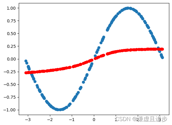
1000次迭代：

3000次迭代：

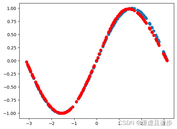
8000次迭代：

20000次迭代：

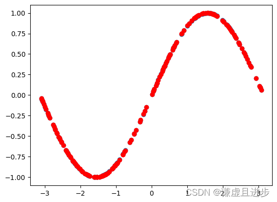
可以看到，20000次迭代之后，MLP完美逼近了sin(x)。而且不是通过有监督回归得到的。参考博客如下：PINN学习与实验（一）__刘文凯_的博客-CSDN博客。

PINN学习与实验之拟合sin(x)

猜你喜欢