深度学习四：tensorflow-使用卷积神经网络识别手写数字

当你安装了tensorflow后，tensorflow自带的教程演示了如何使用卷积神经网络来识别手写数字。代码路径为tensorflow-master\tensorflow\examples\tutorials\mnist\mnist_deep.py。
为了快速测试该程序，我提前将需要的mnist手写数字库下载到了工程目录（我在pycharm中新建了工程，并把mnist_deep.py中的代码拷贝过去）下的input_data目录下：

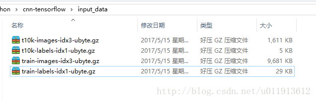
然后，需要修改程序中指定mnist图片库路径的代码，

if __name__ == '__main__':
  print("main run")
  parser = argparse.ArgumentParser()
  parser.add_argument('--data_dir', type=str,
                      **default='input_data'**,
                      help='Directory for storing input data')
  FLAGS, unparsed = parser.parse_known_args()
  tf.app.run(main=main, argv=[sys.argv[0]] + unparsed)

将这里的default的值改为input_data即可。然后程序就可以运行了。默认会训练20000批次，每个批次50个数据。运行完成后准确率达到99.2%。
接下来，这里会对该程序做一点分析，并且做一些修改，来验证一些咱们的猜想，并且加深对代码的理解。

# Copyright 2015 The TensorFlow Authors. All Rights Reserved.
#
# Licensed under the Apache License, Version 2.0 (the "License");
# you may not use this file except in compliance with the License.
# You may obtain a copy of the License at
#
#     http://www.apache.org/licenses/LICENSE-2.0
#
# Unless required by applicable law or agreed to in writing, software
# distributed under the License is distributed on an "AS IS" BASIS,
# WITHOUT WARRANTIES OR CONDITIONS OF ANY KIND, either express or implied.
# See the License for the specific language governing permissions and
# limitations under the License.
# ==============================================================================

"""A deep MNIST classifier using convolutional layers.

See extensive documentation at
https://www.tensorflow.org/get_started/mnist/pros
"""
# Disable linter warnings to maintain consistency with tutorial.
# pylint: disable=invalid-name
# pylint: disable=g-bad-import-order

from __future__ import absolute_import
from __future__ import division
from __future__ import print_function

import argparse
import sys

from tensorflow.examples.tutorials.mnist import input_data

import tensorflow as tf

FLAGS = None


def deepnn(x):
  """deepnn builds the graph for a deep net for classifying digits.

  Args:
    x: an input tensor with the dimensions (N_examples, 784), where 784 is the
    number of pixels in a standard MNIST image.

  Returns:
    A tuple (y, keep_prob). y is a tensor of shape (N_examples, 10), with values
    equal to the logits of classifying the digit into one of 10 classes (the
    digits 0-9). keep_prob is a scalar placeholder for the probability of
    dropout.
  """
  # Reshape to use within a convolutional neural net.
  # Last dimension is for "features" - there is only one here, since images are
  # grayscale -- it would be 3 for an RGB image, 4 for RGBA, etc.
  x_image = tf.reshape(x, [-1, 28, 28, 1])

  # First convolutional layer - maps one grayscale image to 32 feature maps.
  W_conv1 = weight_variable([5, 5, 1, 32])
  b_conv1 = bias_variable([32])
  h_conv1 = tf.nn.relu(conv2d(x_image, W_conv1) + b_conv1)

  # Pooling layer - downsamples by 2X.
  h_pool1 = max_pool_2x2(h_conv1)

  # Second convolutional layer -- maps 32 feature maps to 64.
  W_conv2 = weight_variable([5, 5, 32, 64])
  b_conv2 = bias_variable([64])
  h_conv2 = tf.nn.relu(conv2d(h_pool1, W_conv2) + b_conv2)

  # Second pooling layer.
  h_pool2 = max_pool_2x2(h_conv2)

  # Fully connected layer 1 -- after 2 round of downsampling, our 28x28 image
  # is down to 7x7x64 feature maps -- maps this to 1024 features.
  W_fc1 = weight_variable([7 * 7 * 64, 1024])
  b_fc1 = bias_variable([1024])

  h_pool2_flat = tf.reshape(h_pool2, [-1, 7*7*64])
  h_fc1 = tf.nn.relu(tf.matmul(h_pool2_flat, W_fc1) + b_fc1)

  # Dropout - controls the complexity of the model, prevents co-adaptation of
  # features.
  keep_prob = tf.placeholder(tf.float32)
  h_fc1_drop = tf.nn.dropout(h_fc1, keep_prob)

  # Map the 1024 features to 10 classes, one for each digit
  W_fc2 = weight_variable([1024, 10])
  b_fc2 = bias_variable([10])

  y_conv = tf.matmul(h_fc1_drop, W_fc2) + b_fc2
  return y_conv, keep_prob


def conv2d(x, W):
  """conv2d returns a 2d convolution layer with full stride."""
  return tf.nn.conv2d(x, W, strides=[1, 1, 1, 1], padding='SAME')


def max_pool_2x2(x):
  """max_pool_2x2 downsamples a feature map by 2X."""
  return tf.nn.max_pool(x, ksize=[1, 2, 2, 1],
                        strides=[1, 2, 2, 1], padding='SAME')


def weight_variable(shape):
  """weight_variable generates a weight variable of a given shape."""
  initial = tf.truncated_normal(shape, stddev=0.1)
  return tf.Variable(initial)


def bias_variable(shape):
  """bias_variable generates a bias variable of a given shape."""
  initial = tf.constant(0.1, shape=shape)
  return tf.Variable(initial)


def main(_):
  print("inport data")
  # Import data
  mnist = input_data.read_data_sets(FLAGS.data_dir, one_hot=True)

  # Create the model
  x = tf.placeholder(tf.float32, [None, 784])

  # Define loss and optimizer
  y_ = tf.placeholder(tf.float32, [None, 10])

  # Build the graph for the deep net
  y_conv, keep_prob = deepnn(x)

  cross_entropy = tf.reduce_mean(
      tf.nn.softmax_cross_entropy_with_logits(labels=y_, logits=y_conv))
  train_step = tf.train.AdamOptimizer(1e-4).minimize(cross_entropy)
  correct_prediction = tf.equal(tf.argmax(y_conv, 1), tf.argmax(y_, 1))
  accuracy = tf.reduce_mean(tf.cast(correct_prediction, tf.float32))

  print("start train")
  with tf.Session() as sess:
    sess.run(tf.global_variables_initializer())
    #batch = mnist.train.next_batch(1)
    #print(y_conv.eval(feed_dict={x: batch[0], y_: batch[1], keep_prob: 1.0}))
    for i in range(1000):
      batch = mnist.train.next_batch(50)
      if i % 100 == 0:
        train_accuracy = accuracy.eval(feed_dict={
            x: batch[0], y_: batch[1], keep_prob: 1.0})
        print('step %d, training accuracy %g' % (i, train_accuracy))
      train_step.run(feed_dict={x: batch[0], y_: batch[1], keep_prob: 0.5})

    print('test accuracy %g' % accuracy.eval(feed_dict={
        x: mnist.test.images, y_: mnist.test.labels, keep_prob: 1.0}))


if __name__ == '__main__':
  print("main run")
  parser = argparse.ArgumentParser()
  parser.add_argument('--data_dir', type=str,
                      default='input_data',
                      help='Directory for storing input data')
  FLAGS, unparsed = parser.parse_known_args()
  tf.app.run(main=main, argv=[sys.argv[0]] + unparsed)

这个程序做了如下几点：

第一、装载数据

一开始使用mnist = input_data.read_data_sets(FLAGS.data_dir, one_hot=True)来导入mnist图片库。

第二、使用deepnn函数来构造升经网络

deepnn构造神经网络的过程如下：

2-1 调整输入的图片

 x_image = tf.reshape(x, [-1, 28, 28, 1])

输入的图片本来是一维的，需要把它调整为四维的。-1表示任意多个，两个28指的是图片的长和宽，1是说图片是灰度图，只有一个通道。

2-2构建卷积层

  W_conv1 = weight_variable([5, 5, 1, 32])
  b_conv1 = bias_variable([32])
  h_conv1 = tf.nn.relu(conv2d(x_image, W_conv1) + b_conv1)

weight_variable如下：

def weight_variable(shape):
  """weight_variable generates a weight variable of a given shape."""
  initial = tf.truncated_normal(shape, stddev=0.1)
  return tf.Variable(initial)

其实tensorflow中没有层的概念。tensorflow的整体用一个图表示，可类比为一个神经网络。图则由操作构成。因此这里申明了两个变量，一个是保存权重，一个保存偏执，每一个变量的添加也是一个操作。然后使用tf.nn.relu创建另一个操作。这个操作是一个运算，这个运算首先会计算输入图像与权重的卷积，然后加上偏置，计算完成后，别忘了他是一个激活函数，这个激活函数对权重的卷积加偏置做激活运算。这个过程便是一个神经网络的卷积层所做的事，因此可以看做是一个卷积层。weight_variable的两个5表明卷积核大小为5，1应该还是图像的通道数，32表明该卷积层会提取32个特征，也就是会输出32个maps。
relu是神经元的激活函数，它类似于sigmod,之后我们会对他们做一个对比，看看哪个激活函数有更好的表现。
tf.truncated_normal用来给权重做随机的初始化。

2-3构建池化层

  h_pool1 = max_pool_2x2(h_conv1)

max_pool_2x2函数如下：

def max_pool_2x2(x):
  """max_pool_2x2 downsamples a feature map by 2X."""
  return tf.nn.max_pool(x, ksize=[1, 2, 2, 1],
                        strides=[1, 2, 2, 1], padding='SAME')

ksize是一个四位的结构，第一个参数为1，可以理解为第四维为1，因此它可以理解为一个三维结构了，两个2表明构建池化层的核的大小为2x2,最后的1应该是图像通道数（这里并不确定，如有误，望指正）。strides指的是池化核移动的步幅。参数与ksize相同

2-4全连接层

deepnn构建了两个卷积层，每个卷积层都跟着一个池化层。之后是两个全连接层：

  W_fc1 = weight_variable([7 * 7 * 64, 1024])
  b_fc1 = bias_variable([1024])

  h_pool2_flat = tf.reshape(h_pool2, [-1, 7*7*64])
  h_fc1 = tf.nn.relu(tf.matmul(h_pool2_flat, W_fc1) + b_fc1)

  # Dropout - controls the complexity of the model, prevents co-adaptation of
  # features.
  keep_prob = tf.placeholder(tf.float32)
  h_fc1_drop = tf.nn.dropout(h_fc1, keep_prob)

  # Map the 1024 features to 10 classes, one for each digit
  W_fc2 = weight_variable([1024, 10])
  b_fc2 = bias_variable([10])

  y_conv = tf.matmul(h_fc1_drop, W_fc2) + b_fc2

全连接层的构建只需要指明输入的大小和输出的大小。输入的大小为第二个池化层的所有的输出，输出的大小为1024，也就是这一层有1024个神经元。紧接着又跟了一个大小为10个神经元的全连接层，用来表示10个手写数字。

第三、训练神经网络

  cross_entropy = tf.reduce_mean(
      tf.nn.softmax_cross_entropy_with_logits(labels=y_, logits=y_conv))
  train_step = tf.train.AdamOptimizer(1e-4).minimize(cross_entropy)
  correct_prediction = tf.equal(tf.argmax(y_conv, 1), tf.argmax(y_, 1))
  accuracy = tf.reduce_mean(tf.cast(correct_prediction, tf.float32))

这里使用交叉熵作为误差函数。tf.argmax求一个tensor的最大值的标号，tf.equal用来比对两个标号是否相等。也就是计算出的数字和应该的数字比对是否相等。
tf.train.AdamOptimizer是使用Adam算法的优化器。minimize方法是结合交叉熵代价函数与adam算法，让神经网络的代价不断减少的方法。这个方法其实是compute_gradients()方法和apply_gradients（）方法的组合。Adam的收敛速度会比较快,1e-4是学习速率。
除了Adam算法的优化器外，tensorflow还提供了一些优化器，比如：
class tf.train.GradientDescentOptimizer–梯度下降算法的优化器
class tf.train.AdadeltaOptimizer – 使用adadelta算法的优化器
class tf.train.AdagradOptimizer – 使用adagradOptimizer算法的优化器
class tf.train.MomentumOptimizer – 使用Momentum算法的优化器
等等。大家可以自行尝试那种优化器有更好的效果。
tf.reduce_mean用来计算准确率的平均值。

修改激活函数

关于代码的讲解暂时就说这么多。下面我们做一点尝试，将激活函数改为sigmod:
为了能快速看到结果，以下，我均将训练次数改为了1000次。

inport data
Extracting input_data\train-images-idx3-ubyte.gz
Extracting input_data\train-labels-idx1-ubyte.gz
Extracting input_data\t10k-images-idx3-ubyte.gz
Extracting input_data\t10k-labels-idx1-ubyte.gz
start train
step 0, training accuracy 0.04
step 100, training accuracy 0.08
step 200, training accuracy 0.16
step 300, training accuracy 0.14
step 400, training accuracy 0.34
step 500, training accuracy 0.44
step 600, training accuracy 0.68
step 700, training accuracy 0.7
step 800, training accuracy 0.7
step 900, training accuracy 0.7
test accuracy 0.7732

relu作为激活函数：

main run
inport data
Extracting input_data\train-images-idx3-ubyte.gz
Extracting input_data\train-labels-idx1-ubyte.gz
Extracting input_data\t10k-images-idx3-ubyte.gz
Extracting input_data\t10k-labels-idx1-ubyte.gz
start train
step 0, training accuracy 0.04
step 100, training accuracy 0.86
step 200, training accuracy 0.92
step 300, training accuracy 0.86
step 400, training accuracy 0.96
step 500, training accuracy 0.92
step 600, training accuracy 0.98
step 700, training accuracy 0.96
step 800, training accuracy 0.9
step 900, training accuracy 1
test accuracy 0.9607

可见relu似乎是更好的激活函数

增加卷积层

再增加一个卷积层和一个池化层后，deepnn方法如下：

def deepnn(x):
  """deepnn builds the graph for a deep net for classifying digits.

  Args:
    x: an input tensor with the dimensions (N_examples, 784), where 784 is the
    number of pixels in a standard MNIST image.

  Returns:
    A tuple (y, keep_prob). y is a tensor of shape (N_examples, 10), with values
    equal to the logits of classifying the digit into one of 10 classes (the
    digits 0-9). keep_prob is a scalar placeholder for the probability of
    dropout.
  """
  # Reshape to use within a convolutional neural net.
  # Last dimension is for "features" - there is only one here, since images are
  # grayscale -- it would be 3 for an RGB image, 4 for RGBA, etc.
  x_image = tf.reshape(x, [-1, 28, 28, 1])

  # First convolutional layer - maps one grayscale image to 32 feature maps.
  W_conv1 = weight_variable([5, 5, 1, 32])
  b_conv1 = bias_variable([32])
  h_conv1 = tf.nn.relu(conv2d(x_image, W_conv1) + b_conv1)

  # Pooling layer - downsamples by 2X.
  h_pool1 = max_pool_2x2(h_conv1)

  # Second convolutional layer -- maps 32 feature maps to 64.
  W_conv2 = weight_variable([5, 5, 32, 64])
  b_conv2 = bias_variable([64])
  h_conv2 = tf.nn.relu(conv2d(h_pool1, W_conv2) + b_conv2)

  # Second pooling layer.
  h_pool2 = max_pool_2x2(h_conv2)

  # Second convolutional layer -- maps 32 feature maps to 64.
  W_conv3 = weight_variable([5, 5, 64, 128])
  b_conv3 = bias_variable([128])
  h_conv3 = tf.nn.relu(conv2d(h_pool2, W_conv3) + b_conv3)

  # Second pooling layer.
  h_pool3 = max_pool_2x2(h_conv3)

  # Fully connected layer 1 -- after 2 round of downsampling, our 28x28 image
  # is down to 7x7x64 feature maps -- maps this to 1024 features.
  W_fc1 = weight_variable([4 * 4 * 128, 1024])
  b_fc1 = bias_variable([1024])

  h_pool2_flat = tf.reshape(h_pool3, [-1, 4*4*128])
  h_fc1 = tf.nn.relu(tf.matmul(h_pool2_flat, W_fc1) + b_fc1)

  # Dropout - controls the complexity of the model, prevents co-adaptation of
  # features.
  keep_prob = tf.placeholder(tf.float32)
  h_fc1_drop = tf.nn.dropout(h_fc1, keep_prob)

  # Map the 1024 features to 10 classes, one for each digit
  W_fc2 = weight_variable([1024, 10])
  b_fc2 = bias_variable([10])

  y_conv = tf.matmul(h_fc1_drop, W_fc2) + b_fc2
  return y_conv, keep_prob

训练1000次后：

main run
inport data
Extracting input_data\train-images-idx3-ubyte.gz
Extracting input_data\train-labels-idx1-ubyte.gz
Extracting input_data\t10k-images-idx3-ubyte.gz
Extracting input_data\t10k-labels-idx1-ubyte.gz
start train
step 0, training accuracy 0.06
step 100, training accuracy 0.8
step 200, training accuracy 0.92
step 300, training accuracy 0.84
step 400, training accuracy 0.94
step 500, training accuracy 0.92
step 600, training accuracy 0.98
step 700, training accuracy 0.92
step 800, training accuracy 0.92
step 900, training accuracy 1
test accuracy 0.9624

增加一层卷积层后，效果并没有显著提升。

保存与恢复参数

接下来，保存我们辛辛苦苦训练出来的升经网络的参数：
保存和加载参数主要由类：class tf.train.Saver完成，设计的代码如下：
saver = tf.train.Saver()
save_path = saver.save(sess, model_path)
load_path = saver.restore(sess, model_path)

因此，我们的代码在训练完成后便可将参数保存起来，代码如下：

  **saver = tf.train.Saver()**
  with tf.Session() as sess:
    sess.run(tf.global_variables_initializer())
    #batch = mnist.train.next_batch(1)
    #print(y_conv.eval(feed_dict={x: batch[0], y_: batch[1], keep_prob: 1.0}))
    for i in range(1000):
      batch = mnist.train.next_batch(50)
      if i % 100 == 0:
        train_accuracy = accuracy.eval(feed_dict={
            x: batch[0], y_: batch[1], keep_prob: 1.0})
        print('step %d, training accuracy %g' % (i, train_accuracy))
      train_step.run(feed_dict={x: batch[0], y_: batch[1], keep_prob: 0.5})
    #saver.restore(sess,"./model/me")
    **saver.save(sess,"./model/me")**
    print('test accuracy %g' % accuracy.eval(feed_dict={
        x: mnist.test.images, y_: mnist.test.labels, keep_prob: 1.0}))

下次，我们就不需要再去训练了，我们可以直接加载参数，然后做测试：

  saver = tf.train.Saver()

  with tf.Session() as sess:
    sess.run(tf.global_variables_initializer())
    #batch = mnist.train.next_batch(1)
    #print(y_conv.eval(feed_dict={x: batch[0], y_: batch[1], keep_prob: 1.0}))
    # for i in range(1000):
    #   batch = mnist.train.next_batch(50)
    #   if i % 100 == 0:
    #     train_accuracy = accuracy.eval(feed_dict={
    #         x: batch[0], y_: batch[1], keep_prob: 1.0})
    #     print('step %d, training accuracy %g' % (i, train_accuracy))
    #   train_step.run(feed_dict={x: batch[0], y_: batch[1], keep_prob: 0.5})
    saver.restore(sess,"./model/me")
    #saver.save(sess,"./model/me")
    print('test accuracy %g' % accuracy.eval(feed_dict={
        x: mnist.test.images, y_: mnist.test.labels, keep_prob: 1.0}))

main run
inport data
Extracting input_data\train-images-idx3-ubyte.gz
Extracting input_data\train-labels-idx1-ubyte.gz
Extracting input_data\t10k-images-idx3-ubyte.gz
Extracting input_data\t10k-labels-idx1-ubyte.gz
test accuracy 0.965

直接加载参数后，测试的结果也为0.965