TensorFlow入门之三：tensorflow手写数字识别进阶-卷积神经网络

一、基础知识

基础知识可以跳过，可以直接看后面的代码实现，碰到问题回头来查

1.边界检测示例

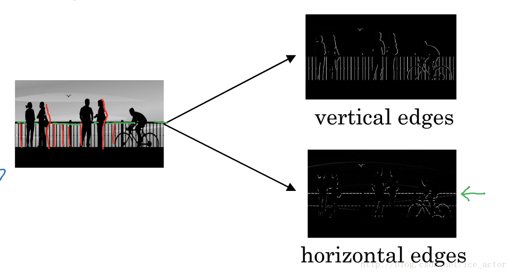
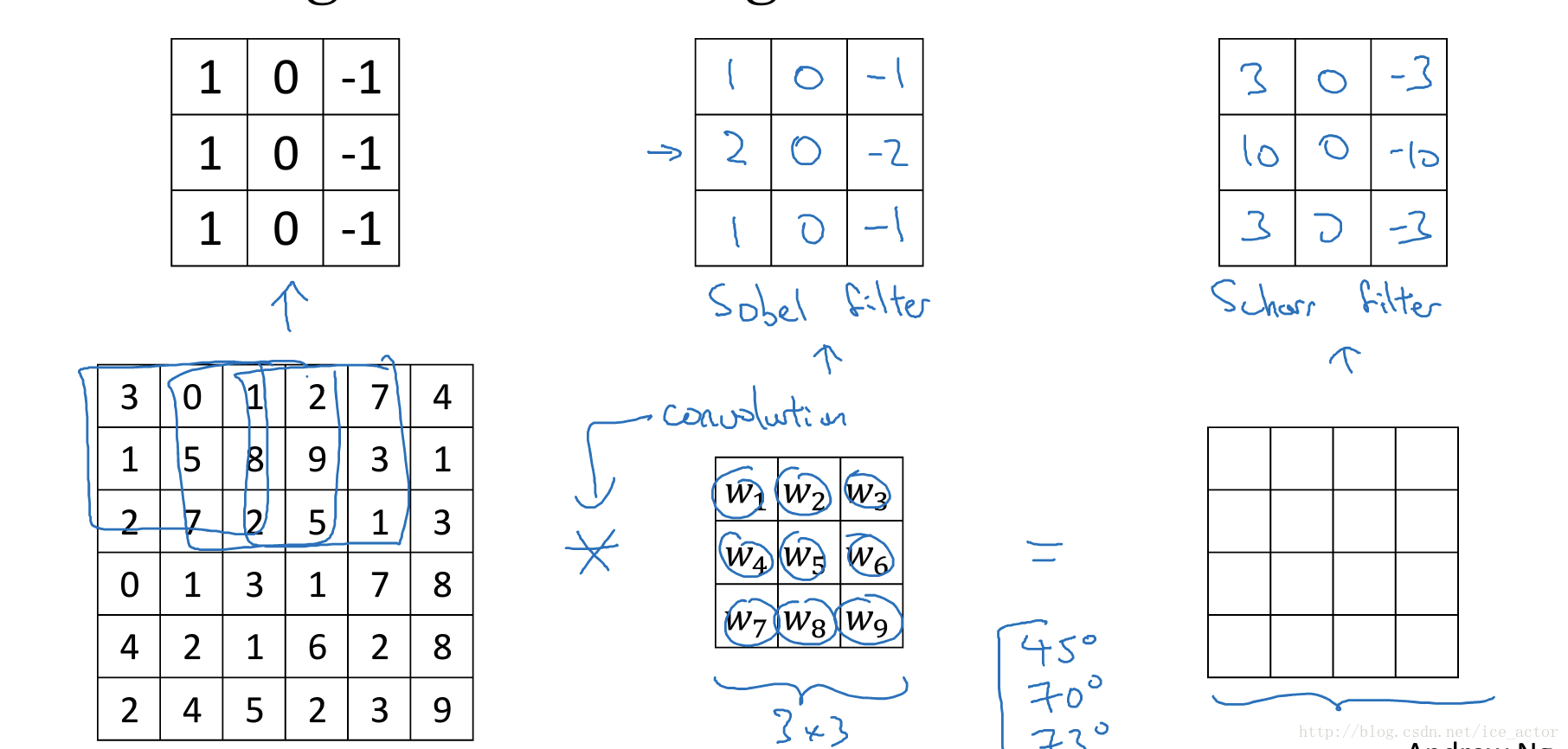
假如你有一张如下的图像，你想让计算机搞清楚图像上有什么物体，你可以做的事情是检测图像的垂直边缘和水平边缘。
这里写图片描述
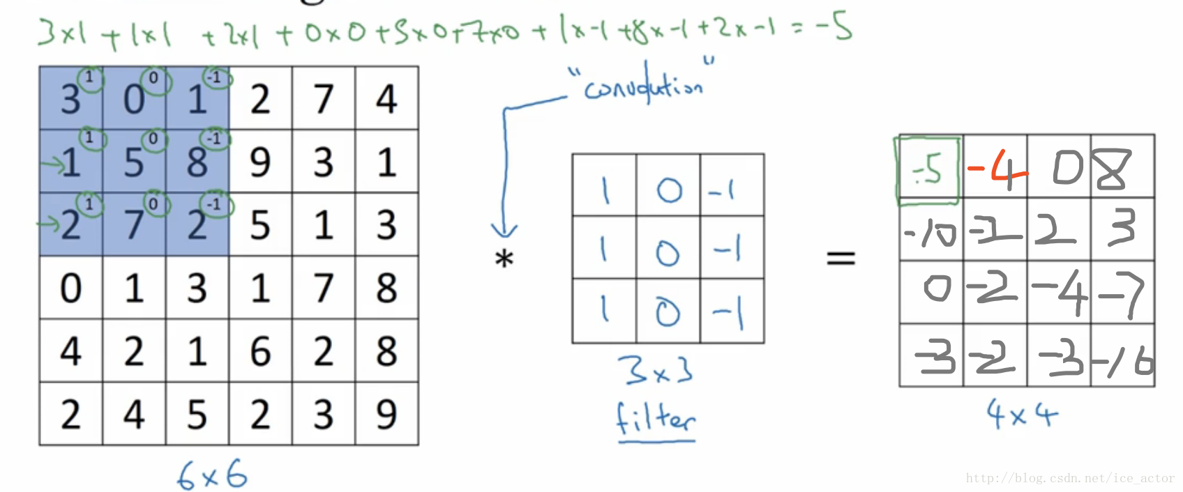
如下是一个6*6的灰度图像，构造一个3*3的矩阵，在卷积神经网络中通常称之为filter，对这个66的图像进行卷积运算，以左上角的-5计算为例
3*1+0*0+1-1+1*1+5*0+8*-1+2*1+7*0+2*-1 = -5
其它的以此类推，让过滤器在图像上逐步滑动，对整个图像进行卷积计算得到一幅44的图像。

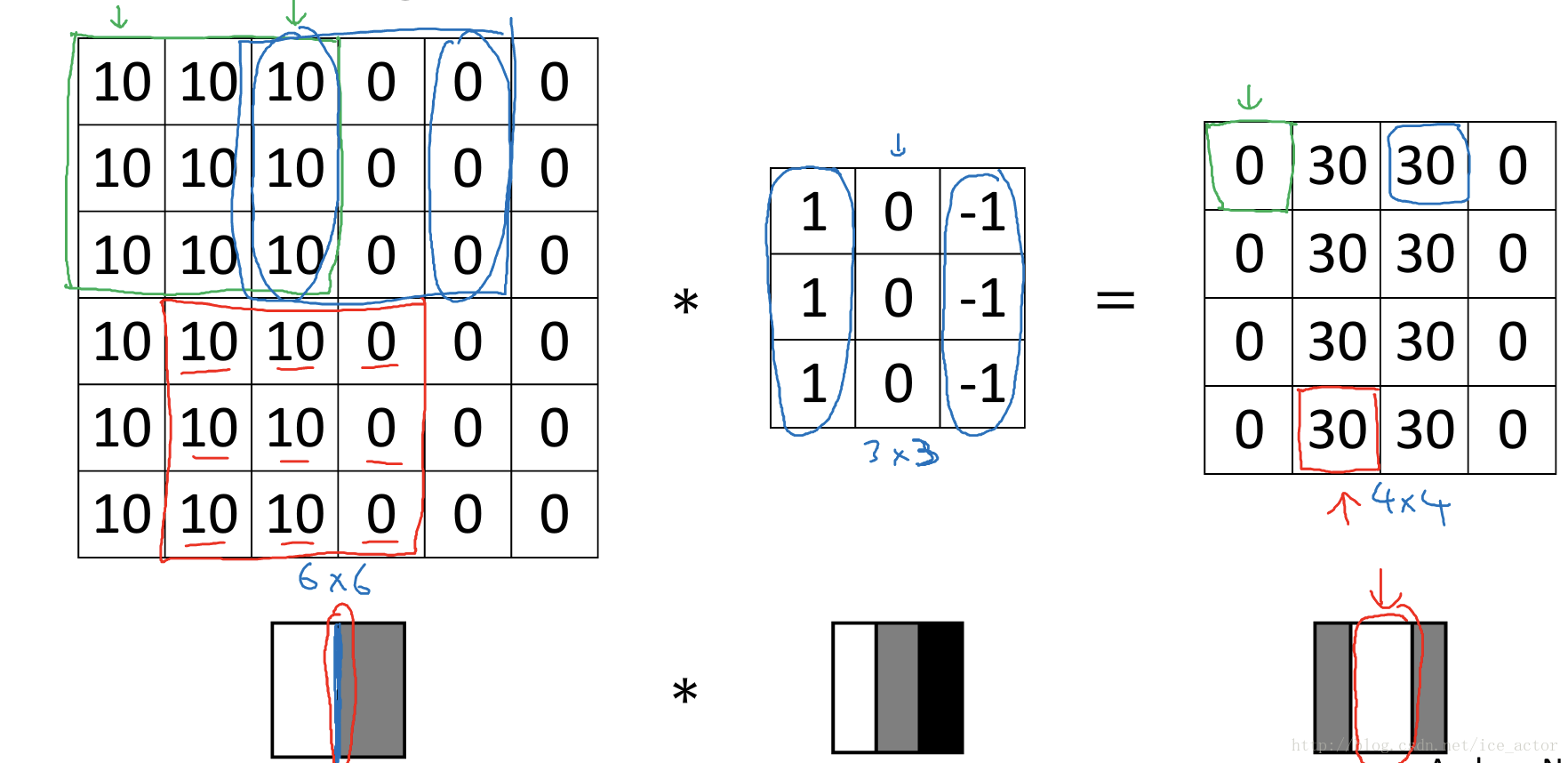
为什么这种卷积计算可以得到图像的边缘，下图0表示图像暗色区域，10为图像比较亮的区域，同样用一个33过滤器，对图像进行卷积，得到的图像中间亮，两边暗，亮色区域就对应图像边缘。
这里写图片描述
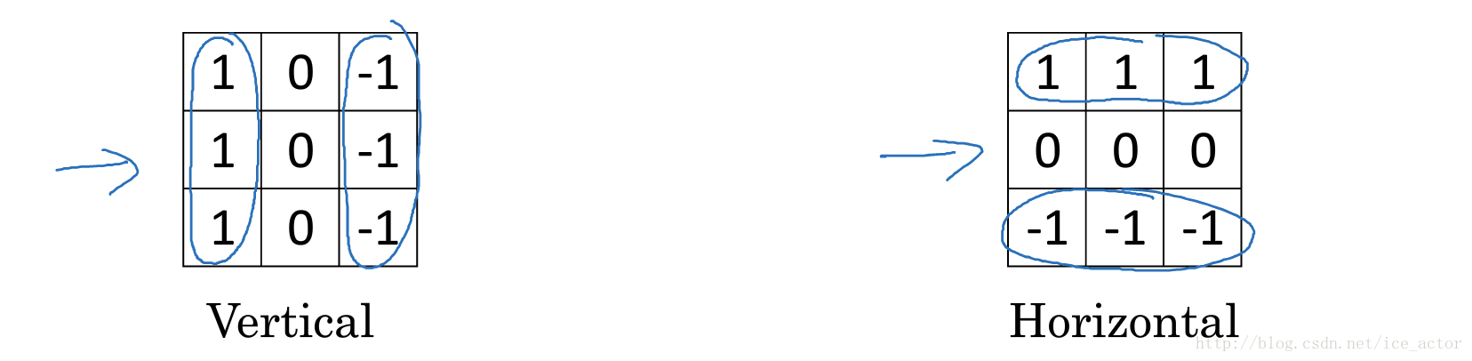
通过以下的水平过滤器和垂直过滤器，可以实现图像水平和垂直边缘检测。

以下列出了一些常用的过滤器，对于不同的过滤器也有着不同的争论，在卷积神经网络中把这些过滤器当成我们要学习的参数，卷积神经网络训练的目标就是去理解过滤器的参数。
这里写图片描述

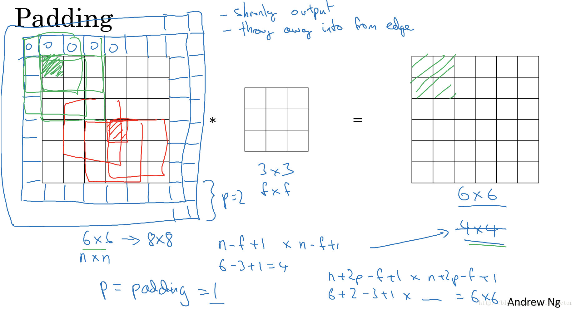
2. padding

在上部分中，通过一个3*3的过滤器来对6*6的图像进行卷积，得到了一幅4*4的图像，假设输出图像大小为n*n与过滤器大小为f*f，输出图像大小则为 $(n−f+1)∗(n−f+1)$ 。
这样做卷积运算的缺点是，卷积图像的大小会不断缩小，另外图像的左上角的元素只被一个输出所使用，所以在图像边缘的像素在输出中采用较少，也就意味着你丢掉了很多图像边缘的信息，为了解决这两个问题，就引入了padding操作，也就是在图像卷积操作之前，沿着图像边缘用0进行图像填充。对于3*3的过滤器，我们填充宽度为1时，就可以保证输出图像和输入图像一样大。
这里写图片描述
padding的两种模式：
Valid：no padding
输入图像n*n,过滤器f*f,输出图像大小为： $(n−f+1)∗(n−f+1)$
Same：输出图像和输入图像一样大

3.卷积步长

卷积步长是指过滤器在图像上滑动的距离，前两部分步长都默认为1，如果卷积步长为2，卷积运算过程为：
这里写图片描述

加入stride后卷积图像大小的通用计算公式为：
输入图像：n*n，过滤器：f*f步长：s，padding：p
输出图像大小为: $\lfloor(\frac{n+2p-f}{s}+1))\rfloor*\lfloor(\frac{n+2p-f}{s}+1)\rfloor$ ， $\lfloor\rfloor$ 表示向下取整

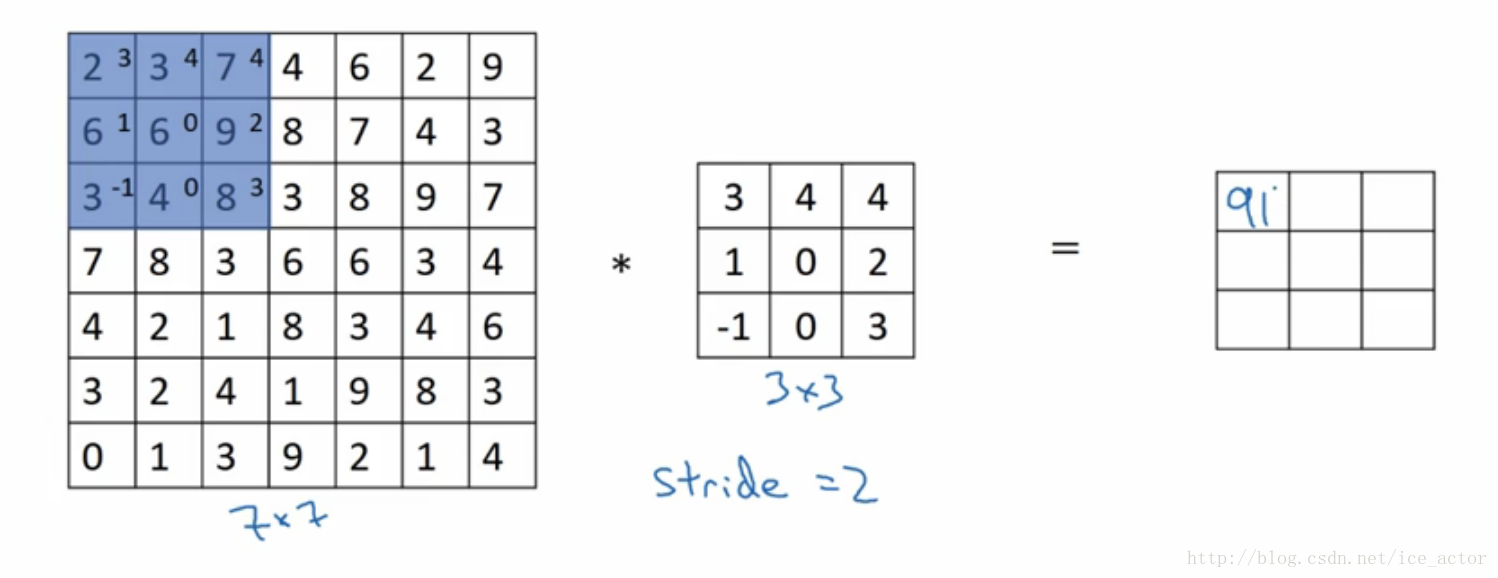
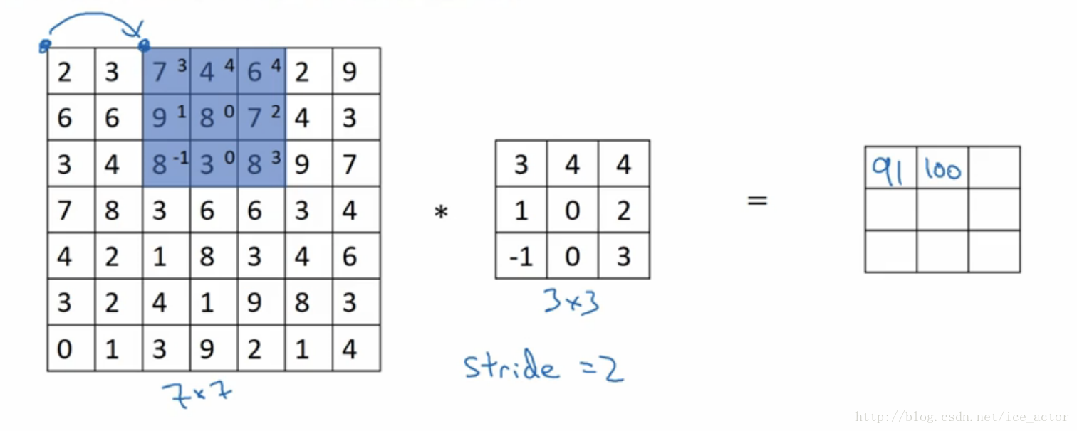
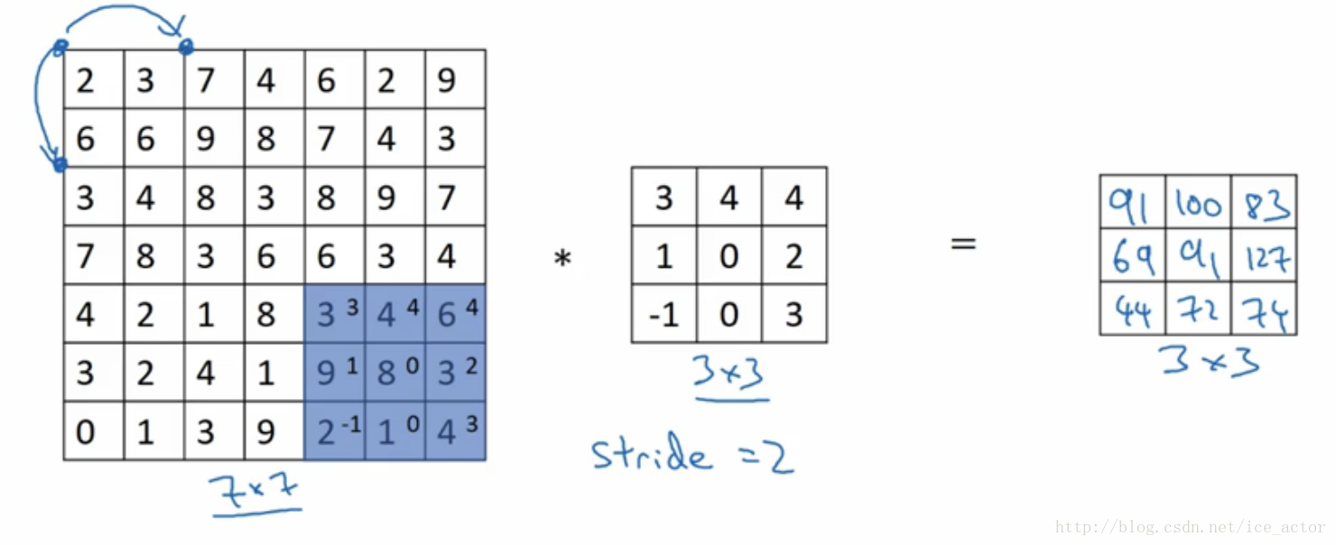
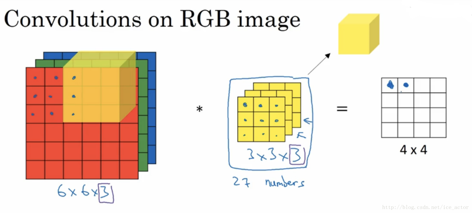
以输入图像7*7，过滤器3*3，步长为2，padding模式为valid为例输出图像大小为: $\lfloor(\frac{7+2*0-3}{2}+1)\rfloor*\lfloor \frac{7+2*0-3}{2}+1)\rfloor=3*3$

4.彩色图像的卷积

以上讲述的卷积都是灰度图像的，如果想要在RGB图像上进行卷积，过滤器的大小不在是3*3而是有3*3*3，最后的3对应为通道数（channels），卷积生成图像中每个像素值为3*3*3过滤器对应位置和图像对应位置相乘累加，过滤器依次在RGB图像上滑动，最终生成图像大小为4*4。
这里写图片描述
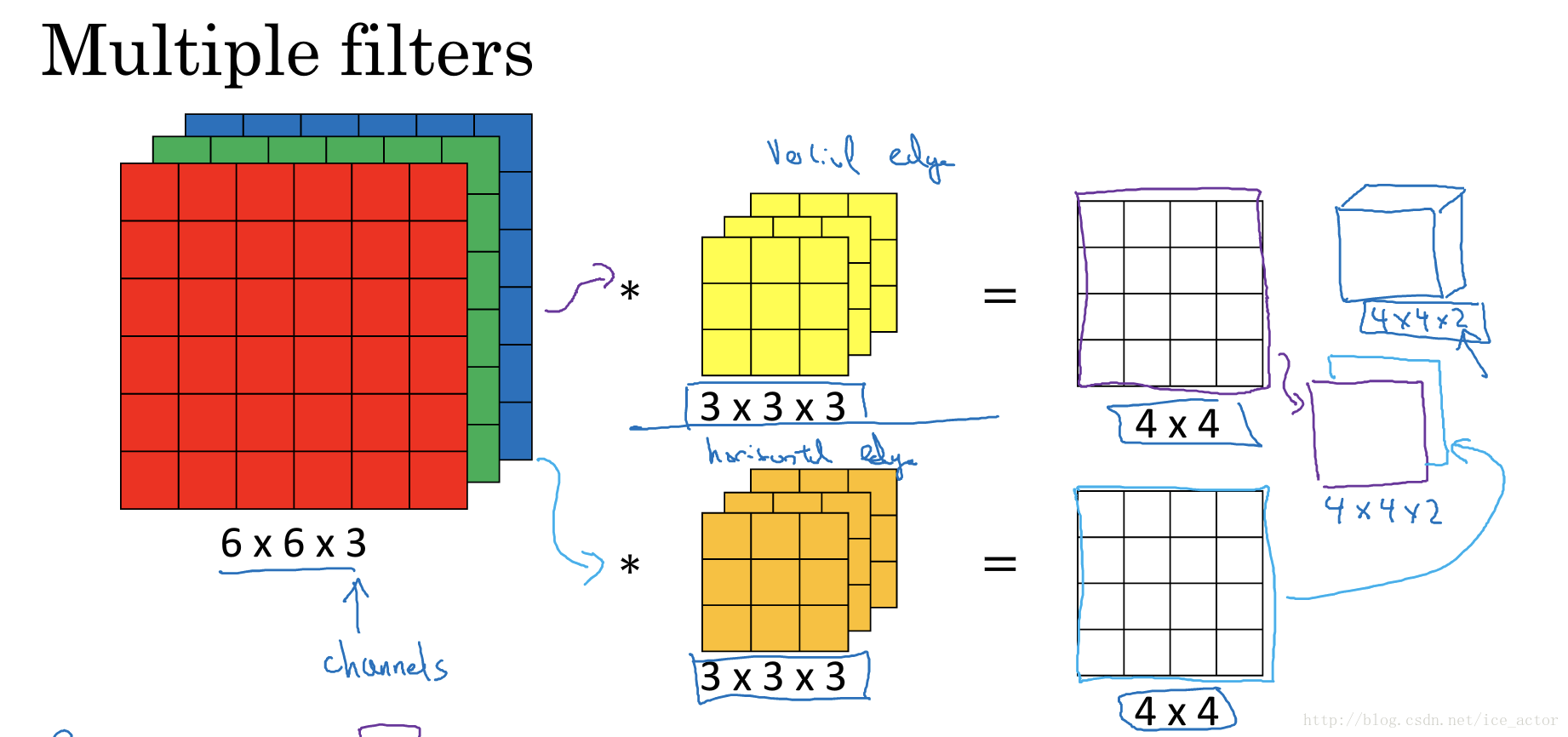
另外一个问题是，如果我们在不仅仅在图像总检测一种类型的特征，而是要同时检测垂直边缘、水平边缘、45度边缘等等，也就是多个过滤器的问题。如果有两个过滤器，最终生成图像为4*4*2的立方体，这里的2来源于我们采用了两个过滤器。如果有10个过滤器那么输出图像就是4*4*10的立方体。
这里写图片描述

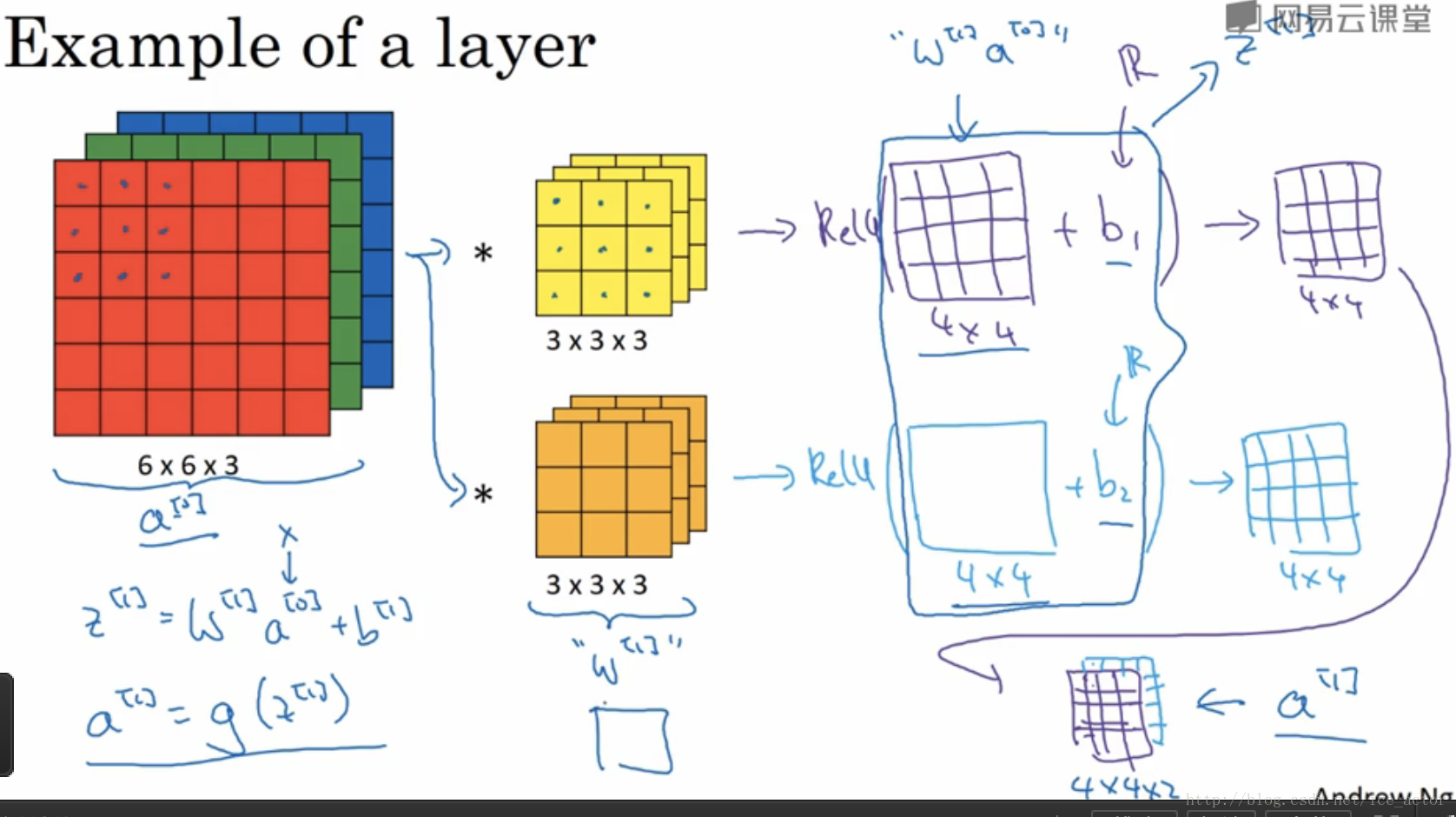
5.单层卷积网络

通过上一节的讲述，图像通过两个过滤器得到了两个44的矩阵，在两个矩阵上分别加入偏差b1b1b_1和b2b2b_2,然后对加入偏差的矩阵做非线性的Relu变换，得到一个新的44矩阵，这就是单层卷积网络的完整计算过程。用公式表示：

$z^{[1]}=w^{[1]}a^{[0]}+b^{[1]}$

$a^{[1]} = g(z^{[1]})$
其中输入图像为 $a^{[0]}$ ,过滤器用 $w^{[1]}$ 表示，对图像进行线性变化并加入偏差得到矩阵 $z^{[1]}$ ， $a^{[1]}$ 是应用Relu激活后的结果。
这里写图片描述

如果有10个过滤器参数个数有多少个呢？
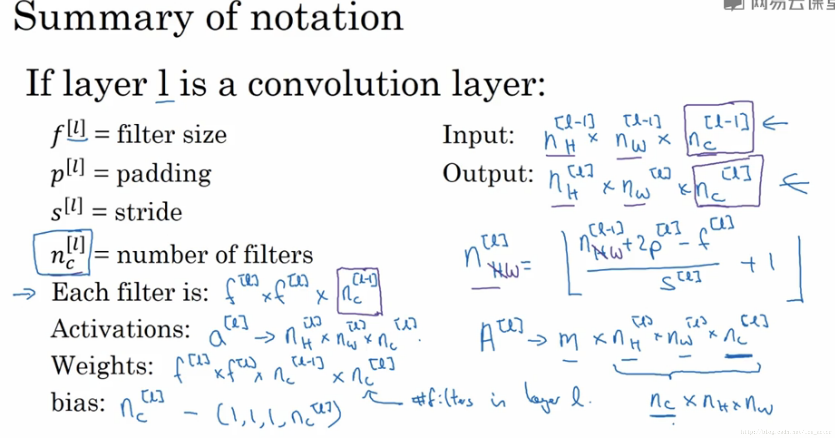
每个过滤器都有3*3*3+1=28个参数，3*3*3为过滤器大小，1是偏差系数，10个过滤器参数个数就是28*10=280个。不论输入图像大小参数个数是不会发生改变的。
描述卷积神经网络的一些符号标识：
lll为一个卷积层：
$f^{[l]}$ ：第 $l$ 层过滤器的大小
$p^{[l]}$ ：第 $l$ 层padding的数量
$s^{[l]}$ ：第 $l$ 层步长大小
$n_C^{l}$ ：过滤器的个数
Input:
$n^{l-1}_{H}\times n^{l-1}_{W}\times n^{l-1}_{C}$ ： $l−1$ 层输入图像的高、宽以及通道数。
Output：
$n^{l}_{H}\times n^{l}_{W}\times n^{l}_{C}$ ：输出图像的高、宽以及通道数
输出图像的大小：
$n_H^{l}=\lfloor\frac{n_H^{l-1}+2*p^{l}-f^{[l]}}{s^l}+1\rfloor$
$n_W^{l}=\lfloor\frac{n_W^{l-1}+2*p^{l}-f^{[l]}}{s^l}+1\rfloor$
输出图像的通道数就是过滤器的个数

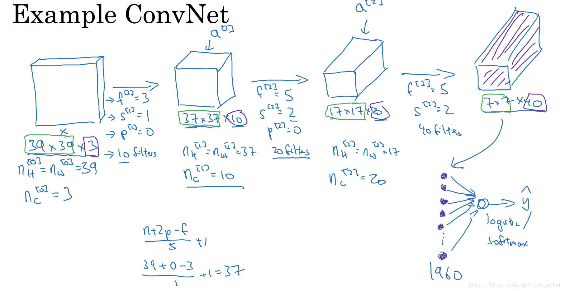
6.简单卷积网络示例

输入图像：39*39*3，padding模式为valid，符号表示： $n_H^{[0]}(高度)=n_W^{[0]}(宽度)=39 ;n_c^{[0]}(颜色通道)=3$
第1层超参数： $f^{[l]}=3$ (过滤器大小)； $s^{[l]}=1$ (步长)； $p^{[l]}=0$ (padding大小)； $n_C^{[l]}=10$ (过滤器个数)
第1层输出图像： $=\lfloor(\frac{39+2*0-3}{1}+1)\rfloor*\lfloor \frac{39+2*0-3}{1}+1)\rfloor=37*37*10$ ，符号表示： $n_H^{[1]}=n_W^{[1]}=37 ;n_c^{[1]}=10$
第2层超参数： $f^{[2]}=5；s^{[2]}=2；p^{[2]}=0；n_C^{[2]}=20$
第2层输出图像： $=\lfloor(\frac{37+2*0-5}{2}+1)\rfloor*\lfloor \frac{37+2*0-5}{2}+1)\rfloor=17*17*20$ ，符号表示： $n_H^{[2]}=n_W^{[2]}=17 ;n_c^{[2]}=20$
第3层超参数： $f^{[3]}=5；s^{[3]}=2；p^{[2]}=0；n_C^{[3]}=40$
第3层输出图像： $=\lfloor(\frac{17+2*0-5}{2}+1)\rfloor*\lfloor \frac{17+2*0-5}{2}+1)\rfloor=7*7*40$ ，符号表示： $n_H^{[3]}=n_W^{[3]}=17 ;n_c^{[3]}=40$
将第三层的输出展开成1960个元素
然后将其输出到logistic或softmax来决定是判断图片中有没有猫，还是想识别图像中K中不同的对象

卷积神经网络层的类型：
卷积层(convolution,conv)
池化层(pooling,pool)
全连接层(Fully connected,FC)

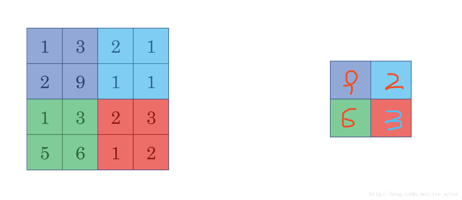
7.池化层

最大池化（Max pooling）
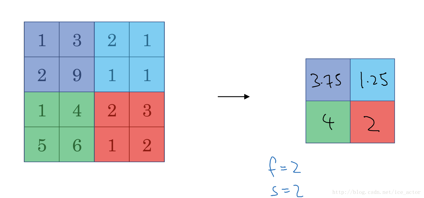
最大池化思想很简单，以下图为例，把4*4的图像分割成4个不同的区域，然后输出每个区域的最大值，这就是最大池化所做的事情。其实这里我们选择了2*2的过滤器，步长为2。在一幅真正的图像中提取最大值可能意味着提取了某些特定特征，比如垂直边缘、一只眼睛等等。
这里写图片描述
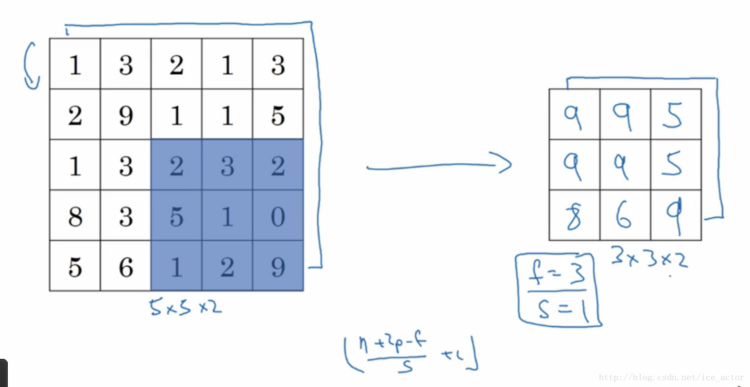
以下是一个过滤器大小为3*3，步长为1的池化过程，具体计算和上面相同，最大池化中输出图像的大小计算方式和卷积网络中计算方法一致，如果有多个通道需要做池化操作，那么就分通道计算池化操作。

平均池化和最大池化唯一的不同是，它计算的是区域内的平均值而最大池化计算的是最大值。在日常应用使用最多的还是最大池化。
这里写图片描述
池化的超参数：步长、过滤器大小、池化类型最大池化or平均池化

8.卷积神经网络示例

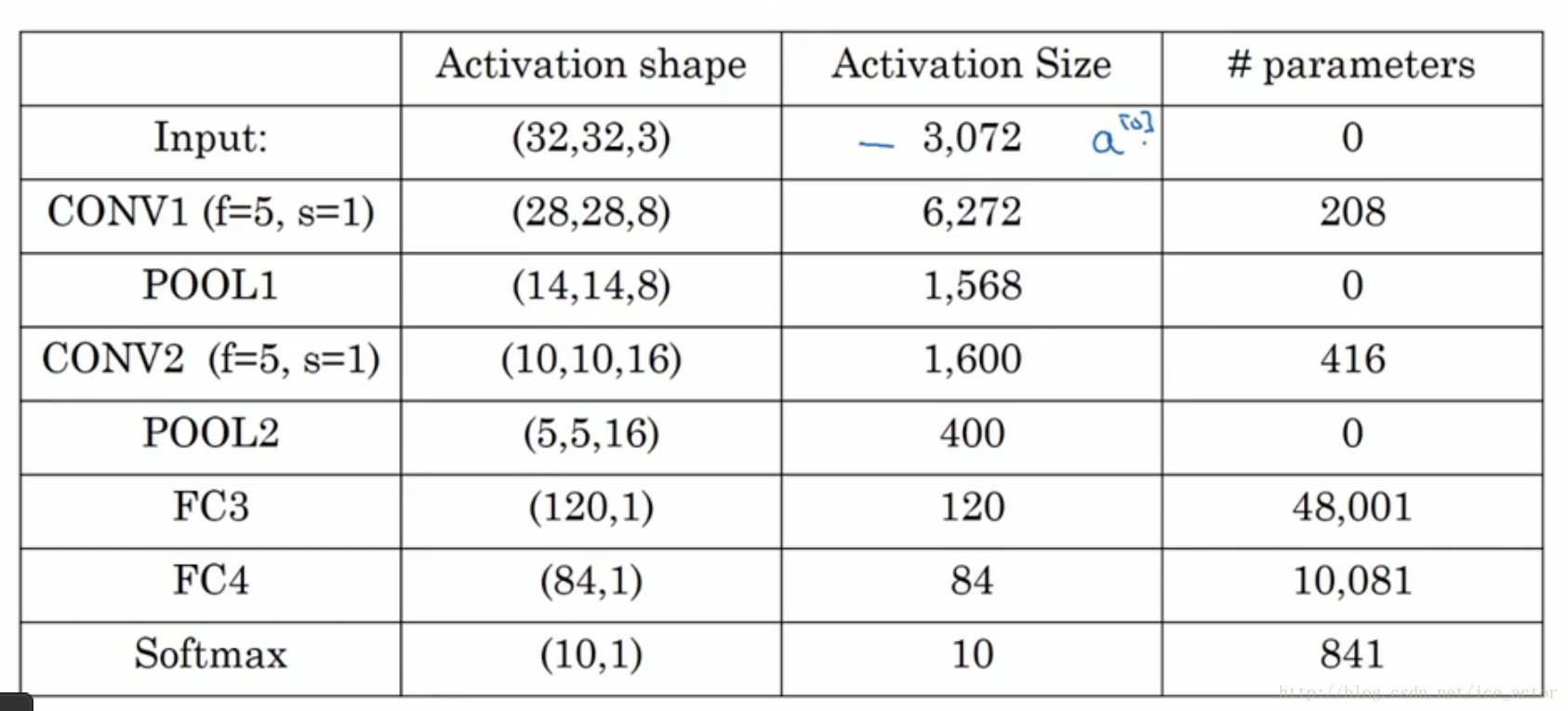
以下是一个完整的卷积神经网络，用于手写字识别，这并不是一个LeNet-5网络，但是设计令该来自于LeNet-5。
这里写图片描述
网络各层参数个数表：

二、使用 TensorFlow 实现卷积神经网络模型

1、网络架构
一个典型的卷积神经网络一般有如下结构：

由于卷积神经网络可以设置的参数非常多，初学者往往无从下手，这里推荐使用成熟的神经网络参数设置，比如LeNet-5、 AlexNet、VGG-16。
2、定义x,y两个Placeholder,把MNIST数据集的训练集数据mnist.train.images及minst.train.labels输入到x,y中。

import tensorflow as tf
import os
import numpy as np
from PIL import Image

x = tf.placeholder("float", shape=[None, 784])
y = tf.placeholder("float", shape=[None, 10])

卷积神经网络的输入一般是3维数据。所以这里需要把输入x转为3维数据。

# 把 X reshape 成 28*28*1的格式,输入的是灰度图片，所有通道数是1;
# shape 里的-1表示数量不定，根据实际情况获取，这里为每轮迭代输入的图像数量（batchsize）的大小;
x_image = tf.reshape(x, [-1,28,28,1])

下面我们打印出来转换的结果x_image

#载入数据集
from tensorflow.examples.tutorials.mnist import input_data
mnist = input_data.read_data_sets("MNIST_data", one_hot=True)
#输出x_image
sess = tf.Session()
batch_xs, batch_ys = mnist.train.next_batch(100)
print(sess.run(x_image, {x: batch_xs, y: batch_ys}))

输出28x28x1的矩阵

[[[[0.]
   [0.]
   [0.]
   ...
   [0.]
   [0.]
   [0.]]
...
  [[0.]
   [0.]
   [0.]
   ...
   [0.]
   [0.]
   [0.]]]]

3、构建第一层的卷积层和池化层。
在神经网络中一般以具有可训练参数的层作为一层，池化层一般是固定参数的，不作为单独一层，和卷积层放在一起称为一层。
这里采用LeNet-5网络的变种。
1). 第一层卷积层的参数如下：
过滤器大小f为5(表示卷积核大小为5x5)，padding模式为same，所以p=5/2=2，步长s为1，卷积核通道n为32。
我们定义这个过滤器：

W_conv1 = tf.Variable(tf.zeros([5,5,1,32]))
b_conv1 = tf.Variable(tf.zeros([32]))

这样全为0的情况，会出现0梯度或者神经元输出恒为0的问题。
由于我们使用的是ReLU神经元，因此比较好的做法是用一个较小的正数来初始化偏置项，比如0.1。
为了创建这个模型，我们需要创建大量的权重和偏置项。我们采用一个函数来实现。这样代码就变成了：

# 全部初始化为0.1
def weight_variable(shape):
  initial = tf.truncated_normal(shape, stddev=0.1)
  return tf.Variable(initial)
  
# 全部初始化为0.1
def bias_variable(shape):
  initial = tf.constant(0.1, shape=shape)
  return tf.Variable(initial)
# [5, 5, 1, 32]里前两个参数表示卷积核尺寸大小，即过滤器大小f;
# 第三个参数是图像通道数，第四个参数是该层卷积核的数量，有多少个卷积核就会输出多少个卷积特征图像
W_conv1 = weight_variable([5, 5, 1, 32])
# 每个卷积核都配置一个偏置量，该层有多少个输出，就应该配置多少个偏置量
b_conv1 = bias_variable([32])

有了这个卷积过滤器，就可以进行卷积操作，代码如下：

# tf.nn.conv2d() 函数实现图片和卷积核卷积操作
# padding='SAME'会对图像边缘补0,完成图像上所有像素（特别是边缘象素）的卷积操作
#strides：卷积时在图像每一维的步长，是一个一维的向量，长度4，并且strides[0]=strides[3]=1
def conv2d(x, W):
  return tf.nn.conv2d(x, W, strides=[1, 1, 1, 1], padding='SAME')

# 将偏置项b_conv1加到卷积结果上去;
# relu激活函数，实现输出结果的非线性转换，即features=max(features, 0)，输出tensor的形状和输入一致
h_conv1 = tf.nn.relu(conv2d(x_image, W_conv1) + b_conv1)

输入28X28X1的矩阵，经过第一层卷积后输出
$=\lfloor(\frac{28+2*2-5}{1}+1)\rfloor*\lfloor \frac{28+2*2-5}{1}+1)\rfloor*32=28*28*32$
padding模式为same，可以不用计算，输出大小和原始图像大小一样，通道数为卷积核数量

2). 第一层池化层的参数固定为f=2，s=2，后面也相同。

# tf.nn.max_pool()函数实现最大池化操作，进一步提取图像的抽象特征，并且降低特征维度
# ksize=[1, 2, 2, 1]定义最大池化操作的核尺寸为2*2
def max_pool_2x2(x):
  return tf.nn.max_pool(x, ksize=[1, 2, 2, 1],
                        strides=[1, 2, 2, 1], padding='SAME')
# 对卷积结果进行池化
h_pool1 = max_pool_2x2(h_conv1)

池化的结果：
$=\lfloor(\frac{28+2*0-2}{2}+1)\rfloor*\lfloor \frac{28+2*0-2}{2}+1)\rfloor*32=14*14*32$
4、构建第二层的卷积层和池化层。
第二层卷积层的参数： $f=5, p=5/2=2, s=1, n=64$
第二层池化层的参数固定为 $f=2，s=2$

#初始化第二层的参数
W_conv2 = weight_variable([5, 5, 32, 64])
b_conv2 = bias_variable([64])
#第二层卷积
h_conv2 = tf.nn.relu(conv2d(h_pool1, W_conv2) + b_conv2)
#第二层池化
h_pool2 = max_pool_2x2(h_conv2)

输入14X14X32的矩阵，经过第一层卷积后输出
$=\lfloor(\frac{14+2*2-5}{1}+1)\rfloor*\lfloor \frac{12+2*2-5}{1}+1)\rfloor*64=14*14*64$
池化后输出
$=\lfloor(\frac{14+2*0-2}{2}+1)\rfloor*\lfloor \frac{14+2*0-2}{2}+1)\rfloor*64=7*7*64$
5、全连接层
现在，图片尺寸减小到7x7，我们加入一个有1024个神经元的全连接层，用于处理整个图片。我们把池化层输出的张量reshape成一些向量1x3136，乘上权重矩阵3136x1024，加上偏置1x1024，然后对其使用ReLU进行非线性变换，得到输出1维向量1x1024。

#二维张量，第一个参数7*7*64的patch，这个参数由最后一层卷积层的输出决定，第二个参数代表卷积个数共1024个，即输出为1024个特征
W_fc1 = weight_variable([7 * 7 * 64, 1024])
# 偏置项为1维，个数跟卷积核个数保持一致
b_fc1 = bias_variable([1024])

#把矩阵7x7x64转为一维向量1x3136
h_pool2_flat = tf.reshape(h_pool2, [-1, 7*7*64])
#把一维向量1x3136和参数矩阵3136x1024相乘，输出1维向量1x1024
#relu激活函数对1维向量进行非线性变黑得到1x1024
h_fc1 = tf.nn.relu(tf.matmul(h_pool2_flat, W_fc1) + b_fc1)

6、Dropout
为了减少过拟合，我们在输出层之前加入dropout。
Dropout机制就是在不同的训练过程中根据一定概率（大小可以设置，一般情况下训练推荐0.5）随机扔掉（屏蔽）一部分神经元，不参与本次神经网络迭代的计算（优化）过程，权重保留但不做更新;
我们用一个placeholder来代表一个神经元的输出在dropout中保持不变的概率。这样我们可以在训练过程中启用dropout，在测试过程中关闭dropout。 TensorFlow的tf.nn.dropout操作除了可以屏蔽神经元的输出外，还会自动处理神经元输出值的scale。所以用dropout的时候可以不用考虑scale。

#keep_prob用于设置概率，需要是一个占位变量，在执行的时候具体给定数值
keep_prob = tf.placeholder("float")
h_fc1_drop = tf.nn.dropout(h_fc1, keep_prob)

7、输出层
最后，我们添加一个softmax层，就像前面的单层softmax regression一样。输入1x1024，乘上权重矩阵1024x10，加上偏移变量1x10，得到1x10的1维向量，然后进行softmax输出概率最高的一个作为输出结果y。

#定义一个输出层参数1024x10
W_fc2 = weight_variable([1024, 10])
#输出层偏移值
b_fc2 = bias_variable([10])

y_conv=tf.nn.softmax(tf.matmul(h_fc1_drop, W_fc2) + b_fc2)

8、我们还是采用交叉熵作为损失函数

loss = -tf.reduce_sum(y*tf.log(y_conv))

9、这里的训练模型，我们采用ADAM优化器来做梯度最速下降。

train_step = tf.train.AdamOptimizer(1e-4).minimize(loss)

10、加上准确率

#计算预测值和实际值是否相等
correct_prediction = tf.equal(tf.argmax(y_conv,1), tf.argmax(y,1))
#对结果求平均值输出准确率
accuracy = tf.reduce_mean(tf.cast(correct_prediction, "float"))

联合起来的程序如下：

import tensorflow as tf
import os
import numpy as np
from PIL import Image
from tensorflow.examples.tutorials.mnist import input_data

#mnist数据集
mnist = input_data.read_data_sets("MNIST_data", one_hot=True)

x = tf.placeholder("float", shape=[None, 784])
y = tf.placeholder("float", shape=[None, 10])

# 把 X reshape 成 28*28*1的格式,输入的是灰度图片，所有通道数是1;
# shape 里的-1表示数量不定，根据实际情况获取，这里为每轮迭代输入的图像数量（batchsize）的大小;
x_image = tf.reshape(x, [-1,28,28,1])

# 参数全部初始化为0.1
def weight_variable(shape):
  initial = tf.truncated_normal(shape, stddev=0.1)
  return tf.Variable(initial)
  
# 偏移值全部初始化为0.1
def bias_variable(shape):
  initial = tf.constant(0.1, shape=shape)
  return tf.Variable(initial)
# [5, 5, 1, 32]里前两个参数表示卷积核尺寸大小，即过滤器大小f;
# 第三个参数是图像通道数，第四个参数是该层卷积核的数量，有多少个卷积核就会输出多少个卷积特征图像
W_conv1 = weight_variable([5, 5, 1, 32])
# 每个卷积核都配置一个偏置量，该层有多少个输出，就应该配置多少个偏置量
b_conv1 = bias_variable([32])

# tf.nn.conv2d() 函数实现图片和卷积核卷积操作
# padding='SAME'会对图像边缘补0,完成图像上所有像素（特别是边缘象素）的卷积操作
#strides：卷积时在图像每一维的步长，是一个一维的向量，长度4，并且strides[0]=strides[3]=1
def conv2d(x, W):
  return tf.nn.conv2d(x, W, strides=[1, 1, 1, 1], padding='SAME')

# 将偏置项b_conv1加到卷积结果上去;
# relu激活函数，实现输出结果的非线性转换，即features=max(features, 0)，输出tensor的形状和输入一致
h_conv1 = tf.nn.relu(conv2d(x_image, W_conv1) + b_conv1)

# tf.nn.max_pool()函数实现最大池化操作，进一步提取图像的抽象特征，并且降低特征维度
# ksize=[1, 2, 2, 1]定义最大池化操作的核尺寸为2*2
def max_pool_2x2(x):
  return tf.nn.max_pool(x, ksize=[1, 2, 2, 1],
                        strides=[1, 2, 2, 1], padding='SAME')
# 对卷积结果进行池化
h_pool1 = max_pool_2x2(h_conv1)

#初始化第二层的参数
W_conv2 = weight_variable([5, 5, 32, 64])
b_conv2 = bias_variable([64])
#第二层卷积
h_conv2 = tf.nn.relu(conv2d(h_pool1, W_conv2) + b_conv2)
#第二层池化
h_pool2 = max_pool_2x2(h_conv2)

#二维张量，第一个参数7*7*64的patch，这个参数由最后一层卷积层的输出决定，第二个参数代表卷积个数共1024个，即输出为1024个特征
W_fc1 = weight_variable([7 * 7 * 64, 1024])
# 偏置项为1维，个数跟卷积核个数保持一致
b_fc1 = bias_variable([1024])

#把矩阵7x7x64转为一维向量1x3136
h_pool2_flat = tf.reshape(h_pool2, [-1, 7*7*64])
#把一维向量1x3136和参数矩阵3136x1024相乘，输出1维向量1x1024
#relu激活函数对1维向量进行非线性变黑得到1x1024
h_fc1 = tf.nn.relu(tf.matmul(h_pool2_flat, W_fc1) + b_fc1)

#keep_prob用于设置概率，需要是一个占位变量，在执行的时候具体给定数值
keep_prob = tf.placeholder("float")
h_fc1_drop = tf.nn.dropout(h_fc1, keep_prob)

#定义一个输出层参数1024x10
W_fc2 = weight_variable([1024, 10])
#输出层偏移值
b_fc2 = bias_variable([10])

#softmax输出预测结果
y_conv=tf.nn.softmax(tf.matmul(h_fc1_drop, W_fc2) + b_fc2)

#交叉熵损失函数
loss = -tf.reduce_sum(y*tf.log(y_conv))

#ADAM优化器来做梯度最速下降
train_step = tf.train.AdamOptimizer(1e-4).minimize(loss)

#计算预测值和实际值是否相等
correct_prediction = tf.equal(tf.argmax(y_conv,1), tf.argmax(y,1))
#对结果求平均值输出准确率
accuracy = tf.reduce_mean(tf.cast(correct_prediction, "float"))

# 创建 Session 用来计算模型
sess = tf.Session()
# 初始化变量
sess.run(tf.initialize_all_variables())

for i in range(20000):
  batch = mnist.train.next_batch(50)
  if i%100 == 0:
    train_accuracy = sess.run(accuracy, feed_dict={
        x:batch[0], y: batch[1], keep_prob: 1.0})
    print("step %d, training accuracy %g"%(i, train_accuracy))
  sess.run(train_step, feed_dict={x: batch[0], y: batch[1], keep_prob: 0.5})

#测试结果
test_batch = mnist.test.next_batch(1000)
test_accuracy = sess.run(accuracy, feed_dict={
    x: test_batch[0], y: test_batch[1], keep_prob: 1.0})
print("test accuracy %g"%test_accuracy)

输出

step 18300, training accuracy 1
step 18400, training accuracy 1
step 18500, training accuracy 1
step 18600, training accuracy 1
step 18700, training accuracy 1
step 18800, training accuracy 1
step 18900, training accuracy 1
step 19000, training accuracy 1
step 19100, training accuracy 1
step 19200, training accuracy 1
step 19300, training accuracy 1
step 19400, training accuracy 1
step 19500, training accuracy 1
step 19600, training accuracy 1
step 19700, training accuracy 1
step 19800, training accuracy 1
step 19900, training accuracy 1
test accuracy 0.992

11、TensorBoard图形化显示
增加代码

# 损失模型隐藏到loss-model模块
with tf.name_scope("loss-model"):
  loss = -tf.reduce_sum(y*tf.log(y_conv))
  # 给损失模型的输出添加scalar，用来观察loss的收敛曲线
  tf.summary.scalar("loss", loss)
...
# 调用 merge_all() 收集所有的操作数据
merged = tf.summary.merge_all()
# 模型运行产生的所有数据保存到 D:/tensorflow 文件夹供 TensorBoard 使用
writer = tf.summary.FileWriter('D:/tensorflow', sess.graph)
    
for i in range(20000):
  batch = mnist.train.next_batch(50)
  if i%100 == 0:
    train_accuracy = sess.run(accuracy, feed_dict={
        x:batch[0], y: batch[1], keep_prob: 1.0})
    print("step %d, training accuracy %g"%(i, train_accuracy))
  # 训练时传入merge
  summary, _ = sess.run([merged, train_step], feed_dict={x: batch[0], y: batch[1], keep_prob: 0.5})
  # 收集每次训练产生的数据
  writer.add_summary(summary, i)

执行显示命令

tensorboard --logdir D:\tensorflow\

然后打开网页http://localhost:6006，可以看到执行流程图

参考：
http://www.tensorfly.cn/tfdoc/tutorials/mnist_pros.html
https://blog.csdn.net/flyfish1986/article/details/79316343
https://blog.csdn.net/ice_actor/article/details/78648780