Ceres简介及示例（9）On Derivatives（Numeric derivatives）

使用analytic derivatives的另一个极端是使用numeric derivatives。关键是，对函数f(x)关于x的求导过程可以写成极限形式:

Forward Differences前向差分

当然，在计算机中，我们不能执行数值求极限操作，所以我们要做的是，选择一个很小的值h并将导数近似为
$\lim_{h \rightarrow 0} \frac{f(x + h) - f(x)}{h}$

上面的公式是数值微分最简单最基本的形式。这就是所谓的前向差分公式。

那么，如何在Ceres求解器中构建Rat43Analytic的数值区分版本呢?这可以通过两个步骤完成:

1.定义给定参数值的Functor，计算给定(x,y)的残差。
2.用NumericDiffCostFunction来构造一个CostFunction来封装实例Rat43CostFunctor。

struct Rat43CostFunctor {
    
    
  Rat43CostFunctor(const double x, const double y) : x_(x), y_(y) {
    
    }

  bool operator()(const double* parameters, double* residuals) const {
    
    
    const double b1 = parameters[0];
    const double b2 = parameters[1];
    const double b3 = parameters[2];
    const double b4 = parameters[3];
    residuals[0] = b1 * pow(1.0 + exp(b2 -  b3 * x_), -1.0 / b4) - y_;
    return true;
  }

  const double x_;
  const double y_;

}
// Analytic算法中手动求解Jacobians的部分被拿掉了。

CostFunction* cost_function =
  new NumericDiffCostFunction<Rat43CostFunctor, FORWARD, 1, 4>(
    new Rat43CostFunctor(x, y));

这是定义成本函数所需的最小工作量。用户需要做的唯一一件事就是确保正确有效地实现了残差的评估。

在进一步深入之前，先对前向差分公式中的误差进行估计是有指导意义的。我们通过考虑f在x附近的泰勒展开式来做。
$\begin{split} f(x+h) &= f(x) + h Df(x) + \frac{h^2}{2!} D^2f(x) + \frac{h^3}{3!}D^3f(x) + \cdots \\ Df(x) &= \frac{f(x + h) - f(x)}{h} - \left [\frac{h}{2!}D^2f(x) + \frac{h^2}{3!}D^3f(x) + \cdots \right]\\ Df(x) &= \frac{f(x + h) - f(x)}{h} + O(h) \end{split}$
即前向差分公式中的误差为O(h)
PS：在渐近误差分析中， $O(h^k)$ 的误差是指当h足够接近0时，误差的绝对值 $h^k$ 最多为的某个常数倍。

实现细节

NumericDiffCostFunction实现了一个普通算法来对给定的仿函数进行数值微分。虽然NumericDiffCostFunction的实际实现很复杂，但最终得到的CostFunction大致如下所示:

class Rat43NumericDiffForward : public SizedCostFunction<1,4> {
    
    
   public:
     Rat43NumericDiffForward(const Rat43Functor* functor) : functor_(functor) {
    
    }
     virtual ~Rat43NumericDiffForward() {
    
    }
     virtual bool Evaluate(double const* const* parameters,
                           double* residuals,
                           double** jacobians) const {
    
    
       functor_(parameters[0], residuals);
       if (!jacobians) return true;
       double* jacobian = jacobians[0];
       if (!jacobian) return true;

       const double f = residuals[0];
       double parameters_plus_h[4];
       for (int i = 0; i < 4; ++i) {
    
    
         std::copy(parameters, parameters + 4, parameters_plus_h);
         const double kRelativeStepSize = 1e-6;
         const double h = std::abs(parameters[i]) * kRelativeStepSize;
         parameters_plus_h[i] += h;
         double f_plus;
         functor_(parameters_plus_h, &f_plus);
         jacobian[i] = (f_plus - f) / h;
       }
       return true;
     }

   private:
     std::unique_ptr<Rat43Functor> functor_;
 };

注意上面代码中步长h的选择，我们使用相对步长 $\text{kRelativeStepSize} = 10^{-6}$ ，而不是对所有参数都相同的绝对步长。
这提供了比绝对步长更好的导数估计。这种步长选择仅适用于不接近于零的参数值。因此，NumericDiffCostFunction的实际实现使用了更复杂的步长选择逻辑，在接近零的地方，它切换到固定的步长。

Central Differences中心差分

O(h)误差在前向差分公式是可以的，但不是很好。一个更好的方法是使用中心差分公式:
$\approx \frac{f(x + h) - f(x - h)}{2h}$

请注意，如果f(x)的值是已知的，Forward Difference公式只需要一个额外的计算，但是Central Difference公式需要两个计算，这使它的成本增加了一倍。
那么，额外的求解值得吗?
为了回答这个问题，我们再次计算中心差分公式中的近似误差:
$\begin{split} f(x + h) &= f(x) + h Df(x) + \frac{h^2}{2!} D^2f(x) + \frac{h^3}{3!} D^3f(x) + \frac{h^4}{4!} D^4f(x) + \cdots\\ f(x - h) &= f(x) - h Df(x) + \frac{h^2}{2!} D^2f(x) - \frac{h^3}{3!} D^3f(c_2) + \frac{h^4}{4!} D^4f(x) + \cdots\\ Df(x) & = \frac{f(x + h) - f(x - h)}{2h} + \frac{h^2}{3!} D^3f(x) + \frac{h^4}{5!} D^5f(x) + \cdots \\ Df(x) & = \frac{f(x + h) - f(x - h)}{2h} + O(h^2) \end{split}$

中心差分公式的误差为 $O(h^2)$ ，即误差以二次形式下降，而正向差分公式中的误差仅以线性形式下降。

在Ceres Solver中使用中心差分而不是前向差分是一个简单的事情，更改NumericDiffCostFunction的模板参数如下

CostFunction* cost_function =
// 将前向差分转换为中心差分很简单：只需要将NumericDiffCostFunction模板参数中的FORWARD更改为CENTRAL
  new NumericDiffCostFunction<Rat43CostFunctor, CENTRAL, 1, 4>(
    new Rat43CostFunctor(x, y));

但是这些误差上的差异在实践中意味着什么呢?为了理解这一点，考虑对单变量函数求导的问题
　　　　　　　　　　　 $\frac{e^x}{\sin x - x^2} ， at x = 1.0$
　　　　　　　　　　　
很容易求出在该位置处的导数 $D f (1.0) = 140.73773557129658$
PS：求导数参考 http://www2.edu-edu.com.cn/lesson_crs78/self/j_0022/soft/ch0302.html

利用这个值作为参考，我们现在可以计算前向和中心差分公式中的相对误差作为绝对步长的函数，并绘制它们。
在这里插入图片描述
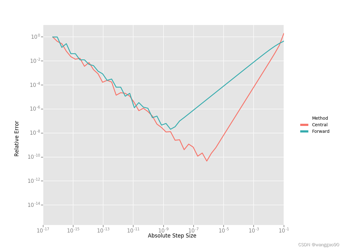
从右到左阅读这张图表，上面的图表中有一些东西很突出:

1.两个公式的图都有两个不同的区域。首先，从一个很大的h值开始，随着截断泰勒级数的影响，这个误差会下降，但是随着h的值继续下降，这个误差开始再次增加，因为“舍入”的误差开始占据计算的主导地位。因此，我们不能继续通过降低h的的方式，获得对Df更精确的估计。我们的近似运算变成了一个明显的限制因素。
2.前向差分公式不是求导的好方法。随着步长的减小，中心差分公式能更快地收敛到更精确的导数估计。因此，除非f(x)的评估函数运算非常复杂以至于中心差分公式无法负担，否则不要使用前向微分公式。
3.对于一个糟糕的h值，这两个公式都不适用。

Ridders’ Method

在上面两种差分方法，精度受到计算机浮点数精度的限制，也就是h不能无限小。那么，我们能否得到更好的对Df的估计，而不需要如此小的h，以至于我们开始碰到浮点数的精度极限？

一种可能的方法是找到一种误差降低得比 $O(h^2)$ 快的方法
这可以通过将Richardson Extrapolation应用到微分问题中来实现。这也被称为Ridders’ Method。

让我们回顾一下，在中心差分公式中的误差。
$\begin{split} Df(x) & = \frac{f(x + h) - f(x - h)}{2h} + \frac{h^2}{3!} D^3f(x) + \frac{h^4}{5!} D^5f(x) + \cdots\\ & = \frac{f(x + h) - f(x - h)}{2h} + K_2 h^2 + K_4 h^4 + \cdots \end{split}$

这里需要注意的关键是 $K_2, K_4, ...$ 与h无关，只与x有关。
让我们定义 $\frac{f(x + h/2^{m-1}) - f(x - h/2^{m-1})}{2h/2^{m-1}}.$

然后观察到 $K_2 h^2 + K_4 h^4 + \cdots \\ Df(x) = A(1, 2) + K_2 (h/2)^2 + K_4 (h/2)^4 + \cdots$

这里我们将步长减半，以获得Df(x)的第二个中心差分估计。结合上面那两种估计，我们得到:
$\frac{4 A(1, 2) - A(1,1)}{4 - 1} + O(h^4)$

它是Df(x)的近似，截断误差为 $O(h^4)$ 但我们不必就此止步。我们可以迭代这个过程，以获得更准确的估计，如下所示:
$\begin{split}A(n, m) = \begin{cases} \frac{\displaystyle f(x + h/2^{m-1}) - f(x - h/2^{m-1})}{\displaystyle 2h/2^{m-1}} & n = 1 \\ \frac{\displaystyle 4^{n-1} A(n - 1, m + 1) - A(n - 1, m)}{\displaystyle 4^{n-1} - 1} & n > 1 \end{cases}\end{split}$

很容易证明 $A (n, 1)$ 的近似误差是 $O(h^{2n})$ 。为了了解上述公式在实际中是如何计算 $A (n, 1)$ 的，可以将计算结构构造为以下表:
$\begin{split}\begin{array}{ccccc} A(1,1) & A(1, 2) & A(1, 3) & A(1, 4) & \cdots\\ & A(2, 1) & A(2, 2) & A(2, 3) & \cdots\\ & & A(3, 1) & A(3, 2) & \cdots\\ & & & A(4, 1) & \cdots \\ & & & & \ddots \end{array}\end{split}$

因此，为了计算 $A (n, 1)$ 对增量n的值，我们从左向右移动，每次计算一列。假设这里的主要代价是对函数f(x)的求值，那么计算上面表中新一列的代价就是两个函数的求值。
由于计算 $A (1, n)$ 的代价，需要计算步长为 $2^{1-n}h$ 的中心差分公式

把这个方法应用到 $\frac{e^x}{\sin x - x^2}$ ，从一个相当大的步长h=0.01开始，我们得到：
$\begin{split}\begin{array}{rrrrr} 141.678097131 &140.971663667 &140.796145400 &140.752333523 &140.741384778\\ &140.736185846 &140.737639311 &140.737729564 &140.737735196\\ & &140.737736209 &140.737735581 &140.737735571\\ & & &140.737735571 &140.737735571\\ & & & &140.737735571\\ \end{array}\end{split}$

相对于参考值 $D f (1.0) = 140.73773557129658 ， A (5, 1)$ 的相对误差为 $10^{-13}$
为比较，在相同步长 $0.01/2^4 = 0.000625$ 下，中心差分公式的相对误差 $0.01/2^4 = 0.000625$

上面的表是Ridders数值微分法的基础。完整的实现是一个自适应方案，它跟踪自己的估计误差，并在达到所需的精度时自动停止。当然，它比前向和中心差分公式更昂贵，但也明显更健壮和准确。
使用Ridder的方法而不是前向或中心差分在Ceres中是一个简单的事情，更改NumericDiffCostFunction的模板参数如下:

CostFunction* cost_function =
  new NumericDiffCostFunction<Rat43CostFunctor, RIDDERS, 1, 4>(
    new Rat43CostFunctor(x, y));

下面的图表显示了使用这三种差分方法时，绝对步长大小与相对误差的关系。对于Ridders的方法，我们假设评估 $A (n, 1)$ 的对应步长为 $2^{1-n}h$ 。

在这里插入图片描述

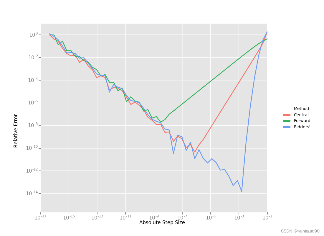
使用Ridders方法计算A(5,1)需要计算十次评估函数，对于Df(1.0)我们的估算结果比中心差分估算好1000倍。为了准确地计算这些数字，计算机的双精度浮点类型 $\approx 2.22 \times 10^{-16}$ 。

回到Rat43，让我们也看看计算数值导数的各种方法的运行时成本

CostFunction	Time (ns)
Rat43Analytic	255
Rat43AnalyticOptimized	92
Rat43NumericDiffForward	262
Rat43NumericDiffCentral	517
Rat43NumericDiffRidders	3760

正如预期的那样，中心差分的运行时间大约是前向差分的两倍，而Ridders方法的运行时间是前两者的好多倍，虽然它的精度也随之显著提高。

建议

当您不能通过分析或使用自动微分来计算导数时，应该使用数值微分。当您调用一个外部库或函数时，通常会出现这种情况，该库或函数的分析形式您不知道，或者即使知道，您也无法以使用Automatic Derivatives的方式重写它。
当使用数值微分时，尽量使用中心差分法。如果不考虑执行时间，或者无法为目标函数确定一个适宜的静态相对步长，那么建议Ridders方法。