使用matlab对图像进行简单处理并分析不同处理方法的特点
对不同曝光程度的图像进行均衡化处理
数据代码段
%直方图均衡化
figure;
srcimage=imread('C:\Users\27019\Desktop\机器视觉\图1-2.jpg');
info=imfinfo('C:\Users\27019\Desktop\机器视觉\图1-2.jpg');
subplot(2,3,1);
imshow(srcimage);
title('原灰度图像');
subplot(2,3,2);
imhist(srcimage);
title('灰度直方图');
subplot(2,3,3);
H1=histeq(srcimage);
imhist(H1);
title('直方图均衡化');
subplot(2,3,4);
histeq(H1);
title('均衡化处理后的图像');
figure;
srcimage=imread(‘C:\Users\27019\Desktop\机器视觉\图1-2.jpg’);
info=imfinfo(‘C:\Users\27019\Desktop\机器视觉\图1-2.jpg’);
subplot(2,3,1);
imshow(srcimage);
title(‘原灰度图像’);
subplot(2,3,2);
imhist(srcimage);
title(‘灰度直方图’);
subplot(2,3,3);
H1=histeq(srcimage);
imhist(H1);
title(‘直方图均衡化’);
subplot(2,3,4);
histeq(H1);
title(‘均衡化处理后的图像’);
分别处理以下三幅图像


这三幅图像分别是灰度范围分布较大,过度曝光和欠曝光的图像。
处理结果如下
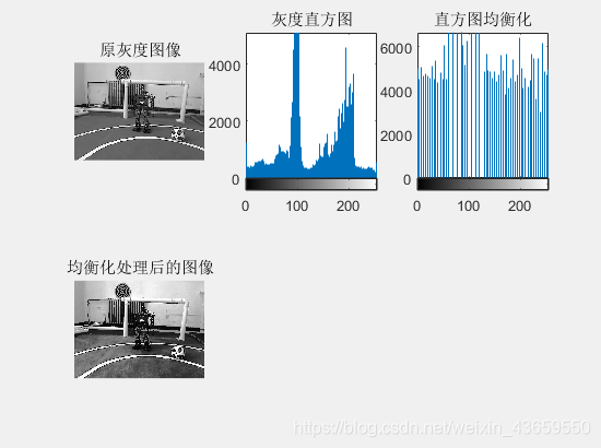
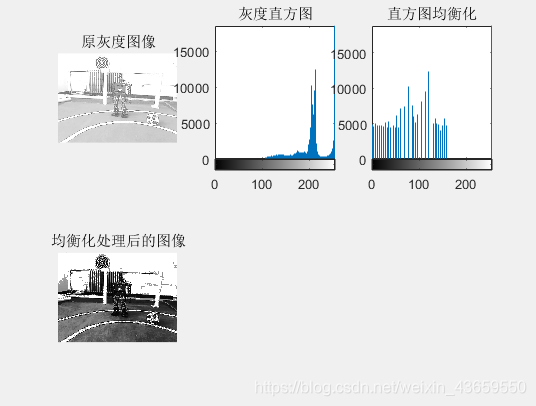
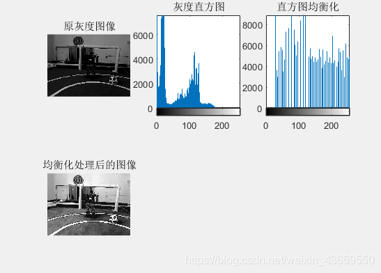
从图像处理的结果来看,主要分别是:过度曝光的图像的灰度直方图大部分集中在灰度值较高的区域,欠曝光的图像的灰度直方图主要集中在灰度值较低的区域,均衡化处理后的直方图分布较为均匀,且图像的亮度较为适中。经过处理后的图像边缘效果更好,图像的信息更明显,达到了增强图像的效果。
对图像进行去噪声处理
使用不同的方法对图像进行去噪声处理,得出各种处理方法的特点。
- 空间域模板卷积(不同模板、不同尺寸)
- 频域低通滤波器(不同滤波模型、不同截止频率)
- 中值滤波方法(不同窗口)
- 均值滤波方法(不同窗口)
备注:对不同方法和同一方法的不同参数的实验结果进行分析和比较,如空间域卷积模板可有高斯型模板、矩形模板、三角形模板和自己根据需求设计的模板等;模板大小可以是3×3,5×5,7×7或更大。频域滤波可采用矩形或巴特沃斯等低通滤波器模型,截止频率也是可选的。
数据代码段
%空间域模板卷积
clc
clear all %清屏
b=imread('C:\Users\27019\Desktop\机器视觉\图1-4.jpg'); %导入图像
a1=double(b)/255;
figure;
subplot(5,3,1),imshow(a1);
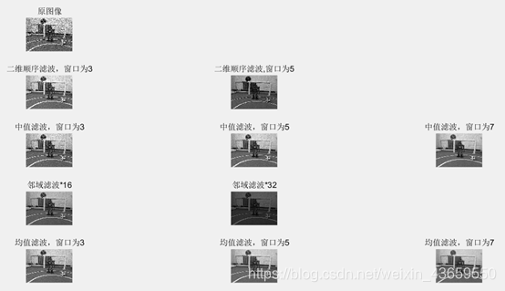
title('原图像');
Q=ordfilt2(b,6,ones(3,3));%二维统计顺序滤波
subplot(5,3,4),imshow(Q);
title('二维顺序滤波,窗口为3')
Q=ordfilt2(b,6,ones(5,5));%二维统计顺序滤波
subplot(5,3,5),imshow(Q);
title('二维顺序滤波,窗口为5')
Q=ordfilt2(b,6,ones(7,7));%二维统计顺序滤波
subplot(5,3,6),imshow(Q);
title('二维顺序滤波,窗口为7')
m=medfilt2(b,[3,3]);%中值滤波
subplot(5,3,7),imshow(m);
title('中值滤波,窗口为3')
m=medfilt2(b,[5,5]);%中值滤波
subplot(5,3,8),imshow(m);
title('中值滤波,窗口为5')
m=medfilt2(b,[7,7]);%中值滤波
subplot(5,3,9),imshow(m);
title('中值滤波,窗口为7')
x=1/16*[0 1 1 1;1 1 1 1;1 1 1 1;1 1 1 0];
a=filter2(x,a1);%邻域滤波*16
subplot(5,3,10),imshow(a);
title('邻域滤波*16')
x=1/32*[0 1 1 1;1 1 1 1;1 1 1 1;1 1 1 0];
a=filter2(x,a1);%邻域滤波*32
subplot(5,3,11),imshow(a);
title('邻域滤波*32')
h = fspecial('average',[3,3]);
A=filter2(h,a1)
subplot(5,3,13),imshow(A);
title('均值滤波,窗口为3')
h = fspecial('average',[5,5]);
A=filter2(h,a1)
subplot(5,3,14),imshow(A);
title('均值滤波,窗口为5')
h = fspecial('average',[7,7]);
A=filter2(h,a1)
subplot(5,3,15),imshow(A);
title('均值滤波,窗口为7')
%高斯模板
figure;
A=imread('C:\Users\27019\Desktop\机器视觉\图1-4.jpg');
subplot(2,3,1);
imshow(A);
title('原始图像');
p=[3,3];
h=fspecial('gaussian',p);
B1=filter2(h,A)/255;
subplot(2,3,2);
imshow(B1);
title('高斯模板,窗口为3');
p=[5,5];
h=fspecial('gaussian',p);
B2=filter2(h,A)/255;
subplot(2,3,3);
imshow(B2);
title('高斯模板,窗口为5');
p=[7,7];
h=fspecial('gaussian',p);
B3=filter2(h,A)/255;
subplot(2,3,4);
imshow(B3);
title('高斯模板,窗口为7');
%均值模板
figure;
A=imread('C:\Users\27019\Desktop\机器视觉\图1-4.jpg');
subplot(2,3,1);
imshow(A);
title('原始图像');
B1=filter2(fspecial('average',3),A)/255;
subplot(2,3,2);
imshow(B1);
title('均值滤波,窗口为3');
B2=filter2(fspecial('average',5),A)/255;
subplot(2,3,3);
imshow(B2);
title('均值滤波,窗口为5');
B3=filter2(fspecial('average',7),A)/255;
subplot(2,3,4);
imshow(B3);
title('均值滤波,窗口为7');
%中值模板
figure;
A=imread('C:\Users\27019\Desktop\机器视觉\图1-4.jpg');
subplot(2,3,1);
imshow(A);
title('原始图像');
B0=medfilt2(A);
subplot(2,3,2);
imshow(B0);
title('中值滤波,窗口为[3,3]');
p=[5,5];
B1=medfilt2(A,p);
subplot(2,3,3);
imshow(B1);
title('中值滤波,窗口为[5,5]');
p=[7,7];
B2=medfilt2(A,p);
subplot(2,3,4);
imshow(B2);
title('中值滤波,窗口为[7,7]');
%空间域模板卷积
clc
clear all %清屏
b=imread(‘C:\Users\27019\Desktop\机器视觉\图1-4.jpg’); %导入图像
a1=double(b)/255;
figure;
subplot(5,3,1),imshow(a1);
title(‘原图像’);
Q=ordfilt2(b,6,ones(3,3));%二维统计顺序滤波
subplot(5,3,4),imshow(Q);
title(‘二维顺序滤波,窗口为3’)
Q=ordfilt2(b,6,ones(5,5));%二维统计顺序滤波
subplot(5,3,5),imshow(Q);
title(‘二维顺序滤波,窗口为5’)
Q=ordfilt2(b,6,ones(7,7));%二维统计顺序滤波
subplot(5,3,6),imshow(Q);
title(‘二维顺序滤波,窗口为7’)
m=medfilt2(b,[3,3]);%中值滤波
subplot(5,3,7),imshow(m);
title(‘中值滤波,窗口为3’)

m=medfilt2(b,[5,5]);%中值滤波
subplot(5,3,8),imshow(m);
title(‘中值滤波,窗口为5’)
m=medfilt2(b,[7,7]);%中值滤波
subplot(5,3,9),imshow(m);
title(‘中值滤波,窗口为7’)
x=1/16*[0 1 1 1;1 1 1 1;1 1 1 1;1 1 1 0];
a=filter2(x,a1);%邻域滤波16
subplot(5,3,10),imshow(a);
title('邻域滤波16’)
x=1/32*[0 1 1 1;1 1 1 1;1 1 1 1;1 1 1 0];
a=filter2(x,a1);%邻域滤波32
subplot(5,3,11),imshow(a);
title('邻域滤波32’)
h = fspecial(‘average’,[3,3]);
A=filter2(h,a1)
subplot(5,3,13),imshow(A);
title(‘均值滤波,窗口为3’)
h = fspecial(‘average’,[5,5]);
A=filter2(h,a1)
subplot(5,3,14),imshow(A);
title(‘均值滤波,窗口为5’)
h = fspecial(‘average’,[7,7]);
A=filter2(h,a1)
subplot(5,3,15),imshow(A);
title(‘均值滤波,窗口为7’)
%高斯模板
figure;
A=imread(‘C:\Users\27019\Desktop\机器视觉\图1-4.jpg’);
subplot(2,3,1);
imshow(A);
title(‘原始图像’);
p=[3,3];
h=fspecial(‘gaussian’,p);
B1=filter2(h,A)/255;
subplot(2,3,2);
imshow(B1);
title(‘高斯模板,窗口为3’);
p=[5,5];
h=fspecial(‘gaussian’,p);
B2=filter2(h,A)/255;
subplot(2,3,3);
imshow(B2);
title(‘高斯模板,窗口为5’);
p=[7,7];
h=fspecial(‘gaussian’,p);
B3=filter2(h,A)/255;
subplot(2,3,4);
imshow(B3);
title(‘高斯模板,窗口为7’);
%均值模板
figure;
A=imread(‘C:\Users\27019\Desktop\机器视觉\图1-4.jpg’);
subplot(2,3,1);
imshow(A);
title(‘原始图像’);
B1=filter2(fspecial(‘average’,3),A)/255;
subplot(2,3,2);
imshow(B1);
title(‘均值滤波,窗口为3’);
B2=filter2(fspecial(‘average’,5),A)/255;
subplot(2,3,3);
imshow(B2);
title(‘均值滤波,窗口为5’);
B3=filter2(fspecial(‘average’,7),A)/255;
subplot(2,3,4);
imshow(B3);
title(‘均值滤波,窗口为7’);
%中值模板
figure;
A=imread(‘C:\Users\27019\Desktop\机器视觉\图1-4.jpg’);
subplot(2,3,1);
imshow(A);
title(‘原始图像’);
B0=medfilt2(A);
subplot(2,3,2);
imshow(B0);
title(‘中值滤波,窗口为[3,3]’);
p=[5,5];
B1=medfilt2(A,p);
subplot(2,3,3);
imshow(B1);
title(‘中值滤波,窗口为[5,5]’);
p=[7,7];
B2=medfilt2(A,p);
subplot(2,3,4);
imshow(B2);
title(‘中值滤波,窗口为[7,7]’);
处理结果如下
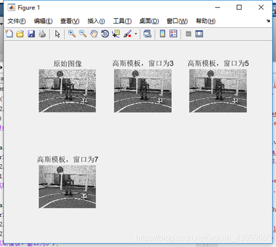
高斯滤波器模型
使用高斯模板滤波得到的图像相比原图像更为清晰,达到了去除噪声的效果。同时当高斯模板的窗口越大,得到的图像会越模糊。

中值滤波方法,窗口为3,5,7
中值滤波原理是使用邻域的中值来代替像素原来的值,得到的图像比较清晰。但是使用的中值滤波方法的窗口越大所得到的图像会越模糊。
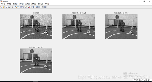
均值滤波方法,窗口为3,5,7
均值滤波可以看出对颗粒的噪声有很好的过滤作用,采用的是使用邻域的均值代替该像素的值。在均值滤波的方法种,窗口越大得到的图像越模糊。
以下几种处理方式在后方处理中重复试用,此处避免累述,只显示结果,分析特点,避免累述
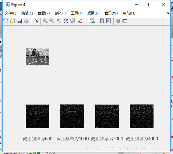
巴特沃斯滤波器模型
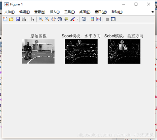
sobel模板
Sobel模板水平和竖直方向上的去噪作用均能达到获取图像的边缘的作用。
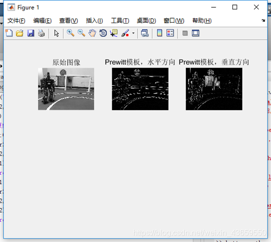
Prewitt模板
Prewitt得到的图像都有突出图像边缘的作用。
图像去噪声结果分析
- 直方图均衡化对哪一类图像增强效果最明显?为什么均衡化后直方图并不平坦?
- 不同空间域卷积器模板的滤波效果有何不同?
- 空间域卷积器模板的大小的滤波效果有何影响?
- 不同频域滤波器的效果有何不同?
回答:
- 对灰度范围分布区间较大的图像的增强效果最明显。这是因为在离散情况下由于灰度取值的离散性不可能把取同一个灰度值的像素变换到不同的像素。也就是说通过灰度直方图均衡化变换函数获得的带有小数的不同灰度值四舍五人取整后会出现归并现象。所以实际应用中就不可能得到完全平坦的直方图但结果图像的灰度直方图相比于原图像直方图要平坦得多。
- 效果最好的是均值滤波,最差的是二维顺序滤波。均值滤波得到的图像比较平滑,而二维顺序滤波得到的图像中还有较多的噪点。中值滤波的图像中仍有一些噪点,领域滤波的图像中亮度偏低。
- 模板越大,图像越模糊,而模板越小,图像越清晰。
- 不同的滤波器得到的图像的滤过的信息不同。
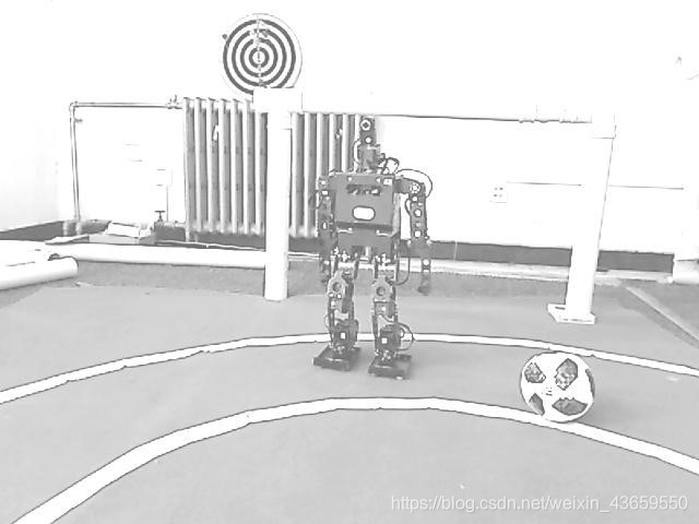
获取内圆,计算距离
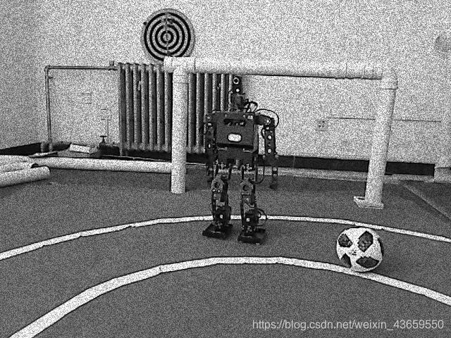
图中一个I-kid机器人A在足球场上拍摄到另一个I-kid机器人B的图片。请首先利用特征提取算法提取地面半径为4.37m的内圆边缘,然后利用所学的摄像机投影模型求解此刻机器人A距离内圆圆心的距离||OA||。(假设机器人A的摄像机被垂直安装,光心位于机器人的中心线上,且其光心距离球场地面为0.5m;同时摄像机的分辨率为640*480像素,主点在其图像中心;摄像机的横向有效焦距为300像素,纵向有效焦距有1200像素)
- 利用Matlab图像工具箱中函数提取图2中球场标记线的内圆边缘。
- 已知图3是球场标志线及机器人A所处大致位置,请利用摄像机线性投影模型计算机器人A离内圆圆心点O的距离||OA||。
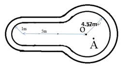
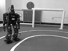
备注:将机器人A的摄像机坐标系先在垂直方向下移0.5m至机器人A的足下,然后平移至圆心点O。从机器人足下平移到圆心O的距离就是待求的距离||OA||。
数据代码段
%Prewitt模板
figure;
A=imread('C:\Users\27019\Desktop\机器视觉\图2.jpg');
subplot(2,3,1);
imshow(A);
title('原始图像');
h=[1 1 1;0 0 0;-1 -1 -1];
B1=filter2(h,A)/255;
subplot(2,3,2);
imshow(B1);
title('Prewitt模板,水平方向');
h=[1 0 -1;1 0 -1;1 0 -1];
B2=filter2(h,A)/255;
subplot(2,3,3)
imshow(B2);
title('Prewitt模板,垂直方向');
%Sobel模板
A=imread('C:\Users\27019\Desktop\机器视觉\图2.jpg');
subplot(2,3,1);
imshow(A);
title('原始图像');
h=[1 2 1;0 0 0;-1 -2 -1];
B1=filter2(h,A)/255;
subplot(2,3,2);
imshow(B1);
title('Prewitt模板,水平方向');
h=[1 0 -1;2 0 -2;1 0 -1];
B2=filter2(h,A)/255;
subplot(2,3,3)
imshow(B2);
title('Prewitt模板,垂直方向');
%低通滤波器
a=imread('C:\Users\27019\Desktop\机器视觉\图1-4.jpg');%读入图像
figure;
subplot(2,4,1);
imshow(a);
z=double(a)/255;
b=fft2(double(a));%对图片进行傅里叶变换
c=log(1+abs(b));
d=fftshift(b);%将变换的原点调整到频率矩阵的中心
e=log(1+abs(d));
%代入巴特沃斯公式进行滤波处理
[m,n]=size(d);
for i=1:256
for j=1:256
d1(i,j)=(1/(1+((i-128)^2+(j-128)^2)^0.5/500)^2)*d(i,j);%截至频率
end;
end;
for i=1:256
for j=1:256
d2(i,j)=(1/(1+((i-128)^2+(j-128)^2)^0.5/1000)^2)*d(i,j);
end;
end;
for i=1:256
for j=1:256
d3(i,j)=(1/(1+((i-128)^2+(j-128)^2)^0.5/2000)^2)*d(i,j);
end;
end;
for i=1:256
for j=1:256
d4(i,j)=(1/(1+((i-128)^2+(j-128)^2)^0.5/4000)^2)*d(i,j);
end;
end;
FF1=ifftshift(d1);
FF2=ifftshift(d2);
FF3=ifftshift(d3);
FF4=ifftshift(d4);
ff1=real(ifft2(FF1));%取傅里叶反变换
ff2=real(ifft2(FF2));
ff3=real(ifft2(FF3));
ff4=real(ifft2(FF4));
subplot(2,4,5);imshow(uint8(ff1));xlabel('截止频率为500');
subplot(2,4,6);imshow(uint8(ff2));xlabel('截止频率为1000');
subplot(2,4,7);imshow(uint8(ff3));xlabel('截止频率为2000');
subplot(2,4,8);imshow(uint8(ff4));xlabel('截止频率为4000');
%不同算子
clear;clc;
close all;
I=imread('C:\Users\27019\Desktop\机器视觉\图2.jpg');
imshow(I,[]);
title('Original Image');
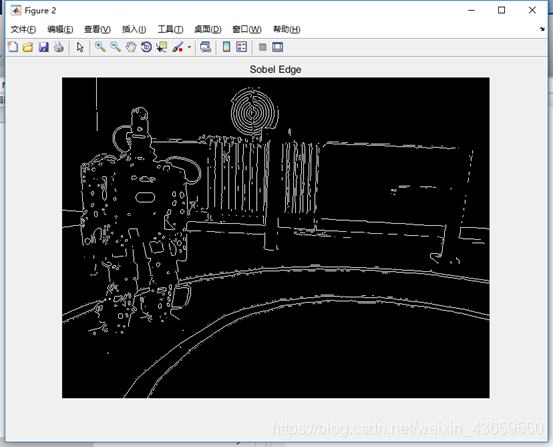
sobelBW=edge(I,'sobel');
figure;
imshow(sobelBW);
title('Sobel Edge');
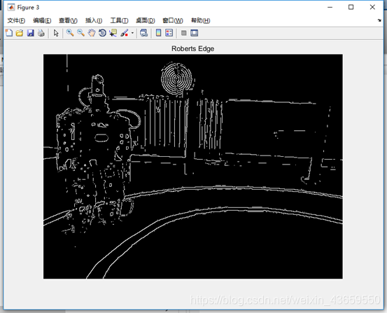
robertsBW=edge(I,'roberts');
figure;
imshow(robertsBW);
title('Roberts Edge');
prewittBW=edge(I,'prewitt');
figure;
imshow(prewittBW);
title('Prewitt Edge');
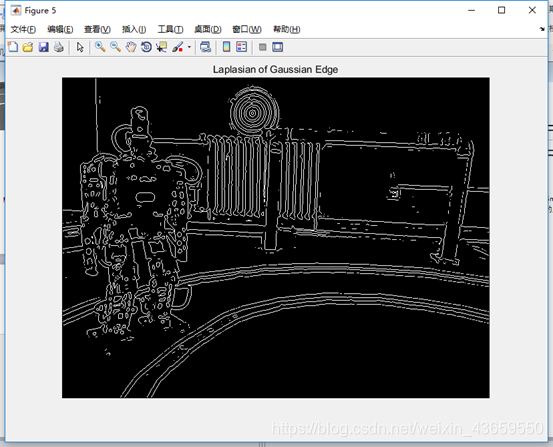
logBW=edge(I,'log');
figure;
imshow(logBW);
title('Laplasian of Gaussian Edge');
cannyBW=edge(I,'canny');
figure;
imshow(cannyBW);
title('Canny Edge');
%标记内圆
img=imread('C:\Users\27019\Desktop\机器视觉\图2.jpg');%读取原图
i=img;
img=im2bw(img); %二值化
[B,L]=bwboundaries(img);
[L,N]=bwlabel(img);
img_rgb=label2rgb(L,'hsv',[.5 .5 .5],'shuffle');
imshow(i);
title('end result')
hold on;
k = 109;
boundary = B{k};
plot(boundary(:,2),boundary(:,1),'y','LineWidth',1);%显示内圆标记线
%Prewitt模板
figure;
A=imread(‘C:\Users\27019\Desktop\机器视觉\图2.jpg’);
subplot(2,3,1);
imshow(A);
title(‘原始图像’);
h=[1 1 1;0 0 0;-1 -1 -1];
B1=filter2(h,A)/255;
subplot(2,3,2);
imshow(B1);
title(‘Prewitt模板,水平方向’);
h=[1 0 -1;1 0 -1;1 0 -1];
B2=filter2(h,A)/255;
subplot(2,3,3)
imshow(B2);
title(‘Prewitt模板,垂直方向’);
%Sobel模板
A=imread(‘C:\Users\27019\Desktop\机器视觉\图2.jpg’);
subplot(2,3,1);
imshow(A);
title(‘原始图像’);
h=[1 2 1;0 0 0;-1 -2 -1];
B1=filter2(h,A)/255;
subplot(2,3,2);
imshow(B1);
title(‘Prewitt模板,水平方向’);
h=[1 0 -1;2 0 -2;1 0 -1];
B2=filter2(h,A)/255;
subplot(2,3,3)
imshow(B2);
title(‘Prewitt模板,垂直方向’);
%低通滤波器
a=imread(‘C:\Users\27019\Desktop\机器视觉\图1-4.jpg’);%读入图像
figure;
subplot(2,4,1);
imshow(a);
z=double(a)/255;
b=fft2(double(a));%对图片进行傅里叶变换
c=log(1+abs(b));
d=fftshift(b);%将变换的原点调整到频率矩阵的中心
e=log(1+abs(d));
%代入巴特沃斯公式进行滤波处理
[m,n]=size(d);
for i=1:256
for j=1:256
d1(i,j)=(1/(1+((i-128)2+(j-128)2)0.5/500)2)*d(i,j);%截至频率
end;
end;
for i=1:256
for j=1:256
d2(i,j)=(1/(1+((i-128)2+(j-128)2)0.5/1000)2)*d(i,j);
end;
end;
for i=1:256
for j=1:256
d3(i,j)=(1/(1+((i-128)2+(j-128)2)0.5/2000)2)*d(i,j);
end;
end;
for i=1:256
for j=1:256
d4(i,j)=(1/(1+((i-128)2+(j-128)2)0.5/4000)2)*d(i,j);
end;
end;
FF1=ifftshift(d1);
FF2=ifftshift(d2);
FF3=ifftshift(d3);
FF4=ifftshift(d4);
ff1=real(ifft2(FF1));%取傅里叶反变换
ff2=real(ifft2(FF2));
ff3=real(ifft2(FF3));
ff4=real(ifft2(FF4));
subplot(2,4,5);imshow(uint8(ff1));xlabel(‘截止频率为500’);
subplot(2,4,6);imshow(uint8(ff2));xlabel(‘截止频率为1000’);
subplot(2,4,7);imshow(uint8(ff3));xlabel(‘截止频率为2000’);
subplot(2,4,8);imshow(uint8(ff4));xlabel(‘截止频率为4000’);
%不同算子
clear;clc;
close all;
I=imread(‘C:\Users\27019\Desktop\机器视觉\图2.jpg’);
imshow(I,[]);
title(‘Original Image’);
sobelBW=edge(I,‘sobel’);
figure;
imshow(sobelBW);
title(‘Sobel Edge’);
robertsBW=edge(I,‘roberts’);
figure;
imshow(robertsBW);
title(‘Roberts Edge’);
prewittBW=edge(I,‘prewitt’);
figure;
imshow(prewittBW);
title(‘Prewitt Edge’);
logBW=edge(I,‘log’);
figure;
imshow(logBW);
title(‘Laplasian of Gaussian Edge’);
cannyBW=edge(I,‘canny’);
figure;
imshow(cannyBW);
title(‘Canny Edge’);
%标记内圆
img=imread(‘C:\Users\27019\Desktop\机器视觉\图2.jpg’);%读取原图
i=img;
img=im2bw(img); %二值化
[B,L]=bwboundaries(img);
[L,N]=bwlabel(img);
img_rgb=label2rgb(L,‘hsv’,[.5 .5 .5],‘shuffle’);
imshow(i);
title(‘end result’)
hold on;
k = 109;
boundary = B{k};
plot(boundary(:,2),boundary(:,1),‘y’,‘LineWidth’,1);%显示内圆标记线
处理结果

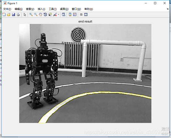
在这里我只做到了标记内圈,计算距离我没能实现,日后实现在评论区补充
结果分析
- 不同边缘提取算子效果有何不同?
- 内圆标记线在图像上为什么不能被拟合为一段标准圆弧?
回答:
- Sobel算子检测方法对灰度渐变和噪声较多的图像处理效果较好。对噪声具有平滑作用,提供较为精确的边缘方向信息,边缘定位精度不够高,图像的边缘不止一个像素。当对精度要求不是很高时,是一种较为常用的边缘检测方法。
Roberts算子检测方法对具有陡峭的低噪声的图像处理效果较好,但是利用roberts算子提取边缘的结果是边缘比较粗,因此边缘的定位不是很准确。
Prewitt算子检测方法对灰度渐变和噪声较多的图像处理效果较好。但边缘较宽,而且间断点多。
Laplacian算子法对噪声比较敏感,所以很少用该算子检测边缘,而是用来判断边缘像素视为与图像的明区还是暗区。
Log算子是高斯滤波和拉普拉斯边缘检测结合在一- 起的产物,它具有Laplace 算子的所有优点,同时也克服了其对噪声敏感的缺点。
Canny方法不容易受噪声干扰,能够检测到真正的弱边缘。优点在于,使用两种不同的阈直分别检测强边缘和弱边缘,并且当弱边缘和强边缘相连时,才将弱边缘包含在输出图像中。 - 图像拍摄的时候,镜头不是垂直于地面,使得得到的图像有一定的畸变。