#清空
rm(list=ls())
gc()
###生成模拟数据###
#生成100个随机数
library(magrittr)
set.seed(1)
asd<-rnorm(100, mean = 60, sd = 10) %>% round #平均60,标准差10
#将10个数随机替换为NA
NA_positions <- sample(1:100, 10)
asd[NA_positions] <- NA
#转化为data.frame
asd <-asd %>% data.frame
colnames(asd)<-"Age"
set.seed(1)
#添加其他相关数据
asd$Weight<-rnorm(100, mean = 75, sd = 5) %>% round
asd$BMI<-rnorm(100,mean=19,sd=4)
asd$Sex<-sample(0:1,100,replace=T) %>% as.factor
asd$death<-sample(0:1,100,replace=T) %>% as.factor
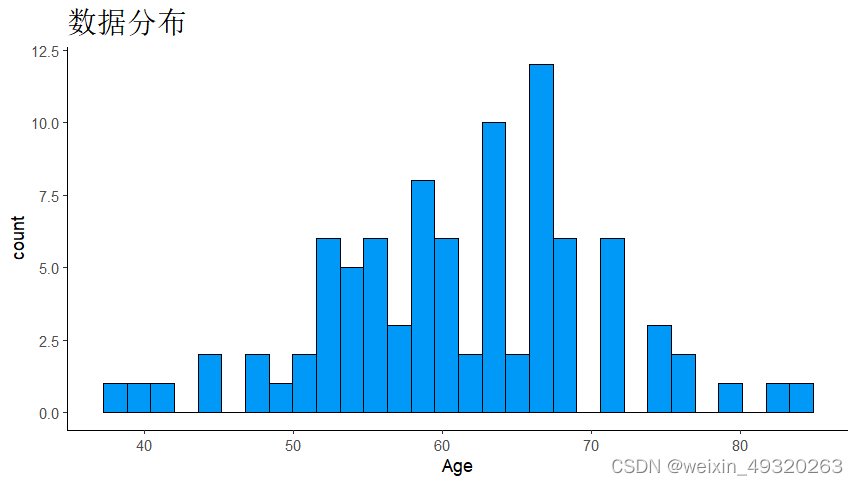
#查看数据分布
str(asd)
library(ggplot2)
ggplot(asd,aes(Age))+#数据集、坐标轴
geom_histogram(color = "#000000", fill = "#0099F8")+#设置直方图线条颜色为黑色,设置直方图填充颜色为蓝色。
ggtitle("数据分布") +#设置坐标轴名称
theme_classic() +#将主题设置为经典风格
theme(plot.title = element_text(size = 18))#将文本字号设置为18
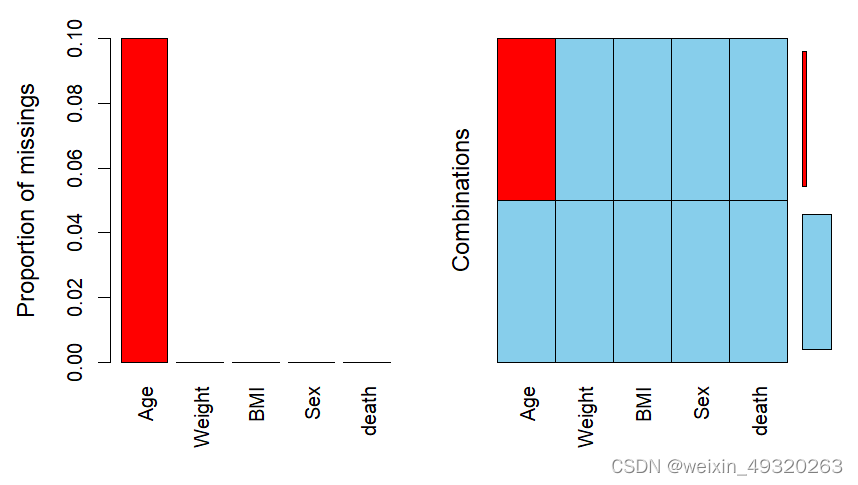
###缺失情况观察###
library(VIM)
aggr(asd,prop=T, numbers=F, sortVars=T)
library(mice)
md.pattern(asd)
###使用 MICE 包进行多重插补缺失值###
library(mice)
help(package="mice")
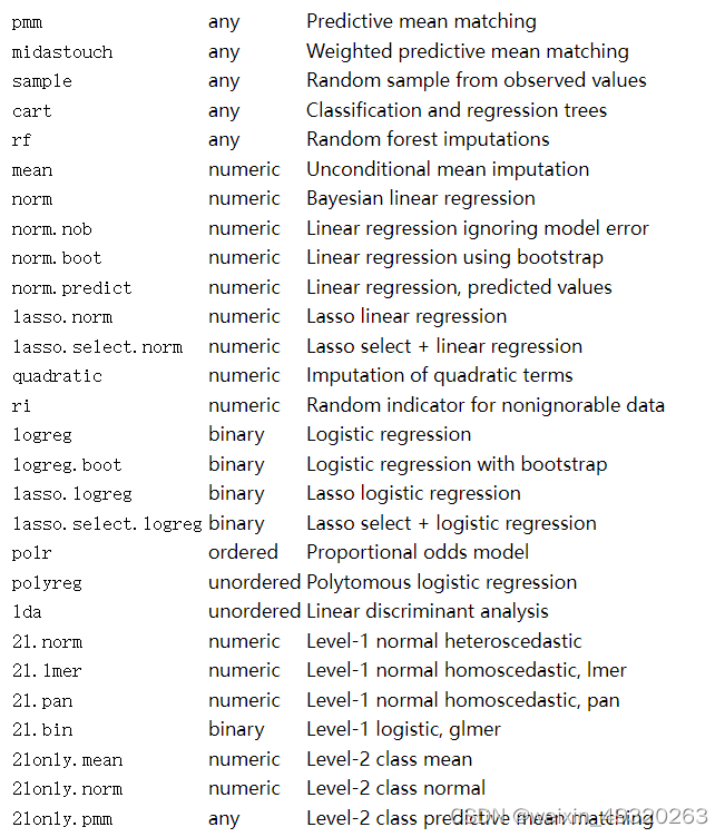
imp_asd<-mice(asd,method="rf",m=10,seed=123)#m代表插补几次
stripplot(imp_asd, cex=1, alpha=1)#可视化插补情况,蓝色是原始数据,红色是插补数据
densityplot(imp_asd)
result<-complete(imp_asd)
###拟合模型###
fit<-with(imp_asd,glm(death~Age+Weight+BMI+Sex,family = binomial))#生成10个回归模型
fit_combine<-pool(fit)#合并10个模型
summary(fit_combine)#总结


备注:mice包支持的方法: