摘要
本文主要介绍Logistic回归,以及Logistic回归在数据集上的应用。
目录
一、问题描述
疝气病一直是牧场主的强敌。牧场主辛勤劳作若干年,将牛、马养的肥肥的,但一旦马患上疝气病,马匹将大量死去,造成牧场瘟疫传播,引发更多的动物死去,牧场主血本无归。医院检测马疝气病的一些指标,有的指标比较主观,有的指标难以测量,例如马的疼痛级别。所以现在能否有更加有效的预测
患有疝气病的马的存活的方法是非常重要的。
牧场主得知可以使用Logistic回归来预测患有疝气病的马的存活,但其预测的准确率未知。现在请收集患有疝气病的马的存活的数据集,使用Logistic回归来预测患有疝气病的马的存活,计算其预测的准确率,判断能否使用Logistic回归来预测患有疝气病的马的存活,使得牧场主可以即时地处理马匹,减少牧场损失。
二、数据获取与预处理
2.1 数据的获取
本数据集是患有疝气病的马的存活的数据集,来自2010年1月的UCI机器学习数据库,其中包含368个样本和28个特征。这里的数据集是有30%的数据缺失的。
2.2 数据预处理
在实现算法之前,需要处理缺失的数据。这里使用实数0来替换所有缺失的值,这种方法恰好适用于Logistic回归。因为当特征值为0时,使用Logistic回归相对应的函数值为0.5,是分界线,不会影响结果。
三、算法的简要介绍
3.1 Sigmoid函数
Logistic回归想要得到的函数是,能接受所有的输入然后返回预测的类别,比如,在两类情况下函数应输出类别0或1。sigmoid函数可是胜任这一工作,它像是一个阶跃函数。其公式如下:
其中,
向量w称为回归系数,也就是我们要找到的最佳参数, x是n维的特征向量,是分类器的输入数据。函数在不同坐标尺度下的曲线图:
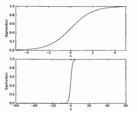
图1 sigmoid函数图像
为了实现Logistic回归分类器,我们可以在每个特征上乘以一个回归系数,然后把所有的结果值相加,将这个总和结果代入sigmoid函数中,进而得到一个范围在0-1之间的数值。
任何大于0.5的数据被分入1类,小于0.5的数据被归入0类。所以,Logistic回归也可以被看成是一种概率估计。
3.2 基于最优化方法的最佳回归系数确定
Sigmoid函数里的一部分: ,其中向量w称为回归系数,也就是我们要找到的最佳参数, x是n维的特征向量,是分类器的输入数据。接下来将介绍几种需找最佳参数的方法:
3.2.1梯度上升法
基于的思想是要找到某函数的最大值,最好的方法是沿着该函数的梯度方向探寻。对于一个函数
,其梯度表示方法如下:
该梯度意味着要沿x和y的方向分别移动一定的距离,这其实是确立了算法到达每个点后下一步移动的方向。其中,函数 必须要在待计算的点上有定义并且可微。
移动方向确定了,这里我们定义移动的大小为步长,用α表示,用向量来表示的话,梯度上升算法的迭代公式如下:
该公式表明,最佳参数w的结果收到梯度变化和步长α的影响,这个公式将一直被迭代执行,直到满足某个停止条件。
梯度上升法的伪代码如下:
初始化每个回归系数为1
重复R次:
计算整个数据集梯度
使用
更新回归系数的向量
返回回归系数
3.2.2随机梯度上升法
梯度上升算法在处理100个左右的数据集时尚可,但如果有数十亿样本和成千上万的特征,那么该方法的计算复杂度将变得很恐怖。
改进方法为随机梯度上升算法,该方法一次仅用一个样本点来更新回归系数。它占用更少的计算资源,是一种在线算法,可以在数据到来时就完成参数的更新,而不需要重新读取整个数据集来进行批处理运算。一次处理所有的数据被称为批处理。
3.2.3改进的随机梯度
在整个迭代过程中,w的三个参数会不同程度的波动。产生这种现象的原因是存在一些被错分的样本点,这些样本在参与每次迭代的过程中都会引起参数的剧烈变化。
为了避免这种剧烈波动,并改善算法的性能,采用以下策略对随机梯度上升算法做了改进:
(1)在每次迭代时更新步长 的值,使得 的值不断减小,但是不能减少为0,这样做的原因是为了保证在多次迭代后新数据仍然具有一定的影响。
(2)通过随机采取样本来更新回归参数,这种方法将减少周期性的波动,每次随机从列表中取一个值,然后该值会从列表中删除。
3.3 画出分界线
在平面上或超平面上,以 作为分界线,此时有
于是,分界线即是
所以,预测的标签的规则为:
四、测试与计算
4.1 Logistic回归的测试
4.1.1 测试数据集
本测试数据集含有100个数据,每个数据含有2个属性,一个二元值得标签,记为1或0。本数据集原始数据如图2所示:
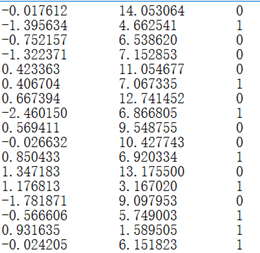
图2 测试数据集
4.1.2计算结果
使用梯度上升法、随机梯度上升法、改进的随机梯度上升法分别进行计算,并且将分界线画出,同时将原始数据集画出,如图3-图6所示。其中,红色表示标签为0的数据,绿色表示标签为1的数据。
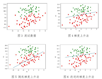
可以看出,梯度上升法的效果较好,分类错误为3个点,但是其计算负复杂度较高。随机梯度上升法的效果很一般,并且错误率明显,有三分之一数据分类错误。改进后的随机梯度上升法有了进步,仅分类错误5个数据。
4.2 问题的计算
上面通过建立Logistic回归模型并进行了测试,其测试结果在可以接受氛围内。所以,现在需要使用Logistic回归模型对患有疝气病的马进行存活的预测。综合了梯度上升法、随机梯度上升法和改进后的随机梯度上升法,由于改进后的随机梯度上升法复杂度较低,并且准确率比随机梯度上升法高,且与梯度上升法的准确率相当,故在此使用改进后的随机梯度上升法进行预测。
通过运行10次来求预测结果的准确率的平均值,其运行结果情况为:
the error rate of this test is: 0.328358
the error rate of this test is: 0.343284
the error rate of this test is: 0.358209
the error rate of this test is: 0.283582
the error rate of this test is: 0.417910
the error rate of this test is: 0.373134
the error rate of this test is: 0.402985
the error rate of this test is: 0.328358
the error rate of this test is: 0.313433
the error rate of this test is: 0.328358
after 10 iterations the average error rate is: 0.347761
计算所得的其中准确率最高的Logistic模型为:
在此模型的预测下,错误率为28.35%,是10次计算预测中错误率最低的一个模型。但即使如此,我们可以看出,在使用Logistic回归模型仅预测是,其错误率仍然很大,并且达到35%。使用Logistic回归进行对患有疝气病的马进行存活的预测的风险很大,所以不建议牧场主使用。
五、总结
本文就Logistic回归进行了介绍,并且给出了三种求解模型系数的方法:梯度上升法、随机梯度上升法和改进后的随机梯度上升法。其中,梯度上升法准确率高,但是复杂度很高。随机梯度上升法复杂度虽然低,但是其准确率低。改进后的随机梯度上升法复杂度在两者中间,并且准确较高。
本文使用改进后的随机梯度上升法构建Logistic回归模型,并且进行对患有疝气病的马进行存活的预测,其计算结果较一般,所以不建议牧场主使用此方法对患有疝气病的马进行存活的预测。
六、参考文献
[1]周志华.机器学习[M].北京:清华大学出版社,2016.
[2]Peter Harrington.机器学习实战[M].北京:人民邮电出版社,2013.
[3]韩家炜等.数据挖掘概念与技术[M].北京:机械工业出版社,2012.
七、附录
《机器学习实战》的代码,其代码的资源网址为:
https://www.manning.com/books/machine-learning-in-action
其中,logRegres.py文件为:
# -*- coding: utf-8 -*-
"""
Created on Sun Apr 22 09:27:33 2018

@author: Diky
"""
from numpy import *

def loadDataSet():
    dataMat = []; labelMat = []
    fr = open('testSet.txt')
    for line in fr.readlines():
        lineArr = line.strip().split()
        dataMat.append([1.0, float(lineArr[0]), float(lineArr[1])])
        labelMat.append(int(lineArr[2]))
    return dataMat,labelMat

def sigmoid(inX):
    return 1.0/(1+exp(-inX))

def gradAscent(dataMatIn, classLabels):
    dataMatrix = mat(dataMatIn)             #convert to NumPy matrix
    labelMat = mat(classLabels).transpose() #convert to NumPy matrix
    m,n = shape(dataMatrix)
    alpha = 0.001
    maxCycles = 500
    weights = ones((n,1))
    for k in range(maxCycles):              #heavy on matrix operations
        h = sigmoid(dataMatrix*weights)     #matrix mult
        error = (labelMat - h)              #vector subtraction
        weights = weights + alpha * dataMatrix.transpose()* error #matrix mult
    return weights

def plotBestFit(weights):
    import matplotlib.pyplot as plt
    dataMat,labelMat=loadDataSet()
    dataArr = array(dataMat)
    n = shape(dataArr)[0]
    xcord1 = []; ycord1 = []
    xcord2 = []; ycord2 = []
    for i in range(n):
        if int(labelMat[i])== 1:
            xcord1.append(dataArr[i,1]); ycord1.append(dataArr[i,2])
        else:
            xcord2.append(dataArr[i,1]); ycord2.append(dataArr[i,2])
    fig = plt.figure()
    ax = fig.add_subplot(111)
    ax.scatter(xcord1, ycord1, s=30, c='red', marker='s')
    ax.scatter(xcord2, ycord2, s=30, c='green')
    x = arange(-3.0, 3.0, 0.1)
    y = (-weights[0]-weights[1]*x)/weights[2]
    ax.plot(x, y)
    plt.xlabel('X1'); plt.ylabel('X2');
    plt.show()

def stocGradAscent0(dataMatrix, classLabels):
    m,n = shape(dataMatrix)
    alpha = 0.01
    weights = ones(n)   #initialize to all ones
    for i in range(m):
        h = sigmoid(sum(dataMatrix[i]*weights))
        error = classLabels[i] - h
        weights = weights + alpha * error * dataMatrix[i]
    return weights

def stocGradAscent1(dataMatrix, classLabels, numIter=150):
    m,n = shape(dataMatrix)
    weights = ones(n)   #initialize to all ones
    for j in range(numIter):
        dataIndex = list(range(m))
        for i in range(m):
            alpha = 4/(1.0+j+i)+0.0001    #apha decreases with iteration, does not
            randIndex = int(random.uniform(0,len(dataIndex)))#go to 0 because of the constant
            h = sigmoid(sum(dataMatrix[randIndex]*weights))
            error = classLabels[randIndex] - h
            weights = weights + alpha * error * dataMatrix[randIndex]
            del(dataIndex[randIndex])
    #print(weights)
    return weights

def classifyVector(inX, weights):
    prob = sigmoid(sum(inX*weights))
    if prob > 0.5: return 1.0
    else: return 0.0

def colicTest():
    frTrain = open('horseColicTraining.txt'); frTest = open('horseColicTest.txt')
    trainingSet = []; trainingLabels = []
    for line in frTrain.readlines():
        currLine = line.strip().split('\t')
        lineArr =[]
        for i in range(21):
            lineArr.append(float(currLine[i]))
        trainingSet.append(lineArr)
        trainingLabels.append(float(currLine[21]))
    trainWeights = stocGradAscent1(array(trainingSet), trainingLabels, 1000)
    errorCount = 0; numTestVec = 0.0
    for line in frTest.readlines():
        numTestVec += 1.0
        currLine = line.strip().split('\t')
        lineArr =[]
        for i in range(21):
            lineArr.append(float(currLine[i]))
        if int(classifyVector(array(lineArr), trainWeights))!= int(currLine[21]):
            errorCount += 1
    errorRate = (float(errorCount)/numTestVec)
    print("the error rate of this test is: %f" % errorRate )
    return errorRate

def multiTest():
    numTests = 10; errorSum=0.0
    for k in range(numTests):
        errorSum += colicTest()
    print("after %d iterations the average error rate is: %f"
          % (numTests, errorSum/float(numTests)) )
Logistic_main.py文件为:
# -*- coding: utf-8 -*-
"""
Created on Sun Apr 22 09:27:33 2018

@author: Diky
"""

from logRegres import *
from numpy import *

"""
data,label = loadDataSet()
weights = gradAscent(data,label)
plotBestFit(weights.getA())
"""

"""
data,label = loadDataSet()
weights = stocGradAscent0(array(data),label)
plotBestFit(weights)
"""

data,label = loadDataSet()
weights = stocGradAscent1(array(data),label,150)
plotBestFit(weights)


"""
multiTest()
"""