Machine Learning - Coursera week5 cost function and backpropagation 1

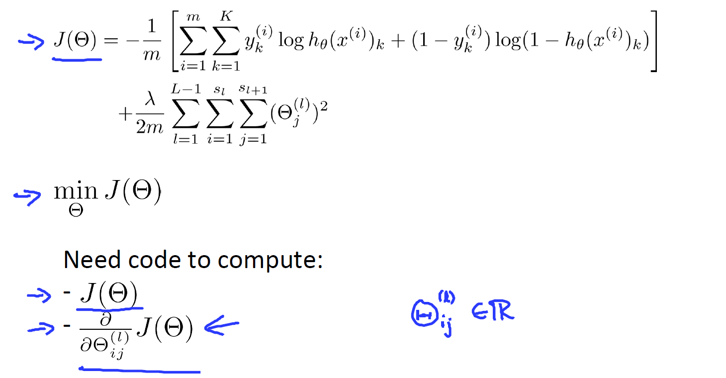
1. cost function

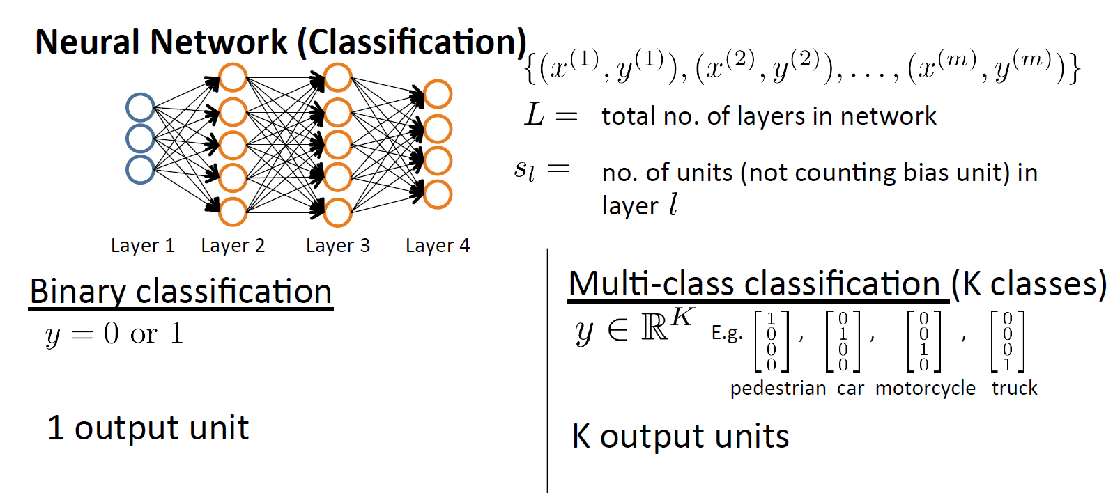
这个多类别分类的神经网络和二分类的输出个数不同，二分类只有一个输出，二多分类模型有多个输出。多分类模型的输出也用one-hot码表示。
变量的定义：
L = total number of layers in the network
$s_l$ = number of units (not counting bias unit) in layer l
K = number of output units/classes
$h_{\theta}(x)_k$=模型的第k个输出

cost function for regularized logistic regression is used ：

$$J(\theta) = \frac{1}{m}\sum_{i=1}^m[-y^{(i)}log(h_{\theta}(x^{(i)})-(1-y^{(i)})log(1-h_{\theta}(x^{(i)})]+\frac{1}{m}\sum_{j=1}^n\theta_j^2$$
For neural networks,
$$\begin{gather*} J(\Theta) = - \frac{1}{m} \sum_{i=1}^m \sum_{k=1}^K \left[y^{(i)}_k \log ((h_\Theta (x^{(i)}))_k) + (1 - y^{(i)}_k)\log (1 - (h_\Theta(x^{(i)}))_k)\right] + \frac{\lambda}{2m}\sum_{l=1}^{L-1} \sum_{i=1}^{s_l} \sum_{j=1}^{s_{l+1}} ( \Theta_{j,i}^{(l)})^2\end{gather*}$$
in the first part,
There is an additional nested summation that loops through the number of output nodes before the square brackets.
in the regularization part,
we must account for multiple theta matrices. The number of columns in our current theta matrix is equal to the number of nodes in our current layer ( including the bias unit). The number of rows in our current theta matrix is equal to the number of nodes in the next layer ( excluding the bias unit).
Note:

• the double sum simply adds up the logistic regression costs calculated for each cell in the output layer
• the triple sum simply adds up the squares of all the individual Θs in the entire network.
• the i in the triple sum does not refer to training example i

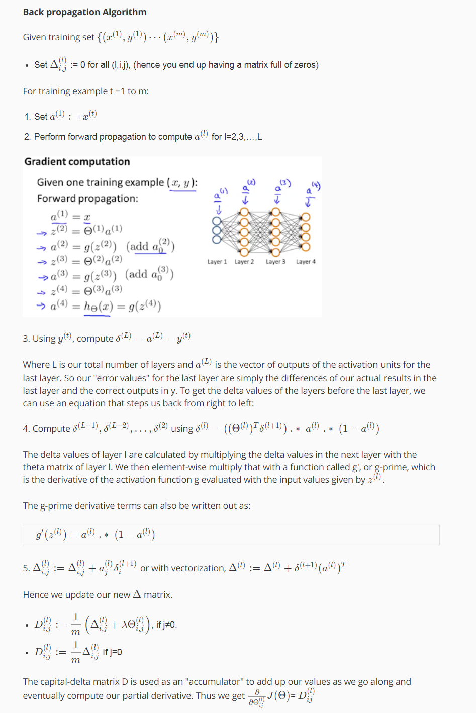
2. backpropagation algorithm

we already have the cost function, What we’d like to do is try to find parameters theta to try to minimize j of theta.
我们使用梯度下降或者更高级的优化算法去求最小值需要求代价函数的偏导数。

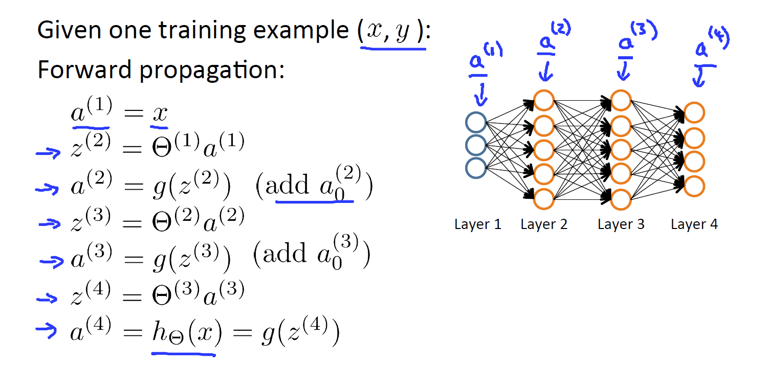
先使用前向传播求出$\theta$的值，激活函数使用sigmoid函数。在向量化计算时，注意添加偏置单元：

反向传播误差的计算就是要计算每一个节点的的误差。具体说来就是l层上第j个节点的误差。比如说第四层的第j个节点的误差可以表示为$\delta_j^{(4)} =a_j^{(4)} - y_j$, $y_j$表示真实的标注。向量化表示为$\delta^{(4)} =a^{(4)} - y$。
接下来就是要理解误差反向传播这个概念。

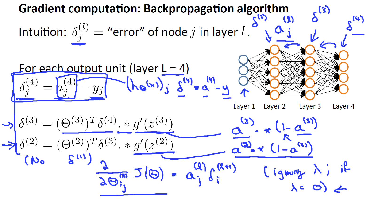
上面我们已经得到了第四层，也就是输出层的误差$\delta^{(4)}$. 我们是要计算每层（除了输入层，我们不需要对输入层考虑误差项 ）上第$j$个节点的误差，那么误差怎么从第四层传播到第三层呢？
从上面的PPT中我们是通过前向传播，把第三层的输出$a^{(3)}$(已加上偏置$a_0^{(3)}$构成第四层的输入)。再有$z^{(4)}=\Theta^{(3)}a^{(3)}$,$a^{(4)}=g(z)$得到的第四层的输出。先看看第三层误差计算的表达式再理解其中的每一项是怎么回事。第三层误差计算的表达式$\delta^{(3)}=(\Theta^{(3)})^T\delta^{(4)}.*g^{'}(z^{(3)})$.第一项很好理解，第四层的误差乘以第四层到第三层的权重$(\Theta^{(3)})^T\delta^{(4)}$,后面的$.*g^{'}(z^{(3)})$如何理解？我没有理解。当我们使用sigmoid函数作为激活函数的时候，导数$g^{'}(z^{(3)})$的结果很美丽，就是$g(z^{(3)}).*(1-g(z^{(3)})$.不理解的话可以看这sigmoid的求导。
误差计算从三层到第二层$\delta^{(2)}=(\Theta^{(2)})^T\delta^{(3)}.*g^{'}(z^{(2)})$。
最后当我们忽略正则项时，我们要求的偏导数恰好就等于激励函数和这些 δ 项，即

$$\frac{\partial J(\theta)}{\partial \Theta_{ij}^{(l)}}=a_j^{(l)}\delta_i^{(l+1)}$$

误差反向传播的计算过程
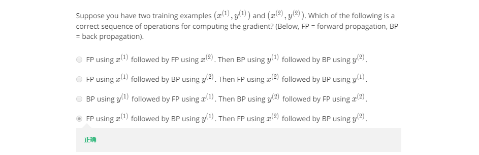
先看一道题：

对每一个样本接下来我们运用正向传播来计算第二层的激励值， 然后是第三层、第四层 ，一直到最后一层 L层。接下来 我们将用这个样本的输出值 y(i) 来计算这个输出值所对应的误差项 δ(L)。 δ(L) 就是模型输出减去实际的标注。接下来 我们将运用反向传播算法来计算 δ(L-1)、δ(L-2)，一直这样直到 δ(2)。再强调一下这里没有 δ(1)，因为我们不需要对输入层考虑误差项。先前向传播然后误差后向传播，再对第二样本进项相同的操作。最后累加我们在前面写好的偏导数： $Δ_{ij}^{(l)}=Δ_{ij}^{(l)}+a_j^{(l)}\delta_i^{(l+1)}$ 使用向量化的形式就是$Δ^{(l)}=Δ^{(l)}+\delta^{(l+1)}(a^{(l)})^T$。 如下

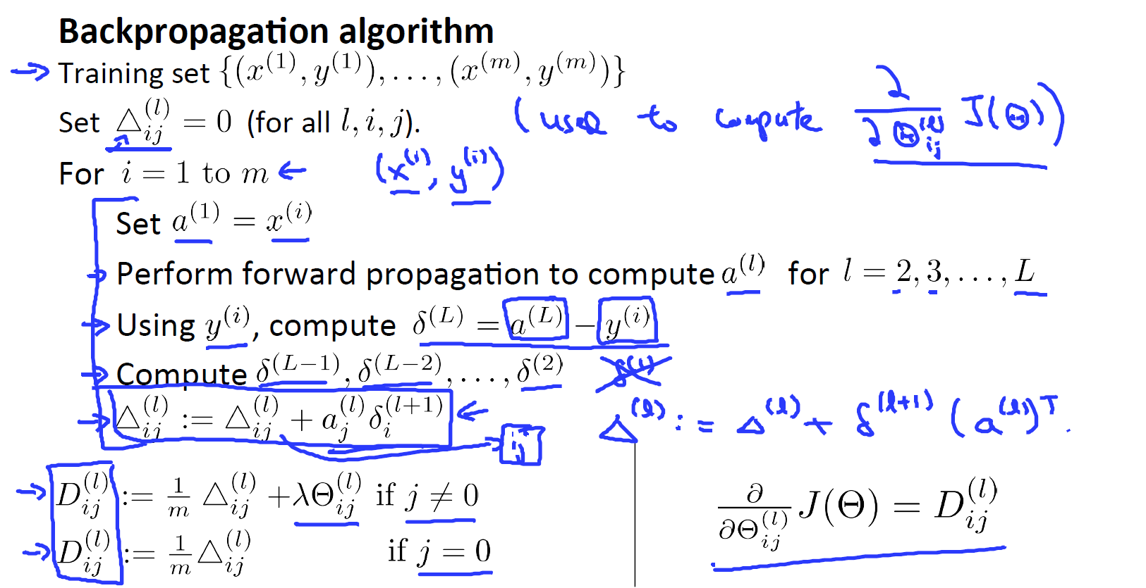
分开考虑有没有正则项的情况，最后我们就得到了我们要求的偏导项。

反向传播的流程