在实习的时候,做的基本上都是没有类标的数据,这让经常在实验室用带类标的数据做实验的我很是头疼。主要是为了熟悉聚类的一些方法,下面介绍聚类以及相应的实现方法,大部分都是别人写的,只是看过后收集整理。
什么是聚类?
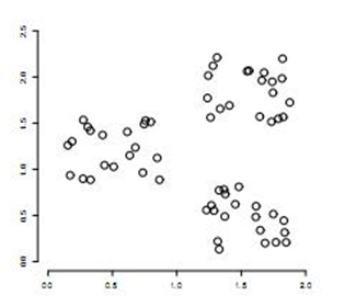
聚类简单的说就是要把一个文档集合根据文档的相似性把文档分成若干类,但是究竟分成多少类,这个要取决于文档集合里文档自身的性质。下面这个图就是一个简单的例子,我们可以把不同的文档聚合为3类。另外聚类是典型的无指导学习,所谓无指导学习是指不需要有人干预,无须人为文档进行标注。
1.先介绍kmeans
kmeans默认是欧式距离,因为要涉及到平均值的计算。
聚类算法:from sklearn.cluster import KMeans
def __init__(self, n_clusters=8, init='k-means++', n_init=10, max_iter=300,tol=1e-4,precompute_distances='auto',verbose=0, random_state=None, copy_x=True, n_jobs=1):(一)输入参数:
(1)n_clusters:要分成的簇数也是要生成的质心数
类型:整数型(int)
默认值:8
n_clusters : int, optional, default: 8
The number of clusters to form as well as the number of centroids to generate.
(2)init:初始化质心,
类型:可以是function 可以是array(random or ndarray)
默认值:采用k-means++(一种生成初始质心的算法)
kmeans++:种子点选取的第二种方法。
kmedoids(PAM,Partitioning Around Medoids)
能够解决kmeans对噪声敏感的问题。kmeans寻找种子点的时候计算该类中所有样本的平均值,如果该类中具有较为明显的离群点,会造成种子点与期望偏差过大。例如,A(1,1),B(2,2),C(3,3),D(1000,1000),显然D点会拉动种子点向其偏移。这样,在下一轮迭代时,将大量不该属于该类的样本点错误的划入该类。
为了解决这个问题,kmedoids方法采取新的种子点选取方式,1)只从样本点中选;2)选取标准能够提高聚类效果,例如上述的最小化J函数,或者自定义其他的代价函数。但是,kmedoids方法提高了聚类的复杂度。
init : {'k-means++', 'random' or an ndarray}
Method for initialization, defaults to 'k-means++':
'k-means++' : selects initial cluster centers for k-mean clustering in a smart way to speed up convergence. See section Notes in k_init for more details.
(3)n_init: 设置选择质心种子次数,默认为10次。返回质心最好的一次结果(好是指计算时长短)
类型:整数型(int)
默认值:10
目的:每一次算法运行时开始的centroid seeds是随机生成的, 这样得到的结果也可能有好有坏. 所以要运行算法n_init次, 取其中最好的。
n_init : int, default: 10
Number of time the k-means algorithm will be run with different centroid seeds. The final results will be the best output of n_init consecutive runs in terms of inertia.
(4)max_iter:每次迭代的最大次数
类型:整型(int)
默认值:300
max_iter : int, default: 300
Maximum number of iterations of the k-means algorithm for a
single run.
(5)tol: 容忍的最小误差,当误差小于tol就会退出迭代(算法中会依赖数据本身)
类型:浮点型(float)
默认值:le-4(0.0001)
Relative tolerance with regards to inertia to declare convergence
(6)precompute_distances: 这个参数会在空间和时间之间做权衡,如果是True 会把整个距离矩阵都放到内存中,auto 会默认在数据样本大于featurs*samples 的数量大于12e6 的时候False,False时核心实现的方法是利用Cpython 来实现的
类型:布尔型(auto,True,False)
默认值:“auto”
Precompute distances (faster but takes more memory).
'auto' : do not precompute distances if n_samples * n_clusters > 12 million. This corresponds to about 100MB overhead per job usingdouble precision.
(7)verbose:是否输出详细信息
类型:布尔型(True,False)
默认值:False
verbose : boolean, optional
Verbosity mode.
(8)random_state: 随机生成器的种子 ,和初始化中心有关
类型:整型或numpy(RandomState, optional)
默认值:None
random_state : integer or numpy.RandomState, optional
The generator used to initialize the centers. If an integer is given, it fixes the seed. Defaults to the global numpy random number generator.
(9)copy_x:bool 在scikit-learn 很多接口中都会有这个参数的,就是是否对输入数据继续copy 操作,以便不修改用户的输入数据。这个要理解Python 的内存机制才会比较清楚。
类型:布尔型(boolean, optional)
默认值:True
When pre-computing distances it is more numerically accurate to center the data first. If copy_x is True, then the original data is not modified. If False, the original data is modified, and put back before the function returns, but small numerical differences may be introduced by subtracting and then adding the data mean.
(10)n_jobs: 使用进程的数量,与电脑的CPU有关
类型:整数型(int)
默认值:1
The number of jobs to use for the computation. This works by computing
each of the n_init runs in parallel.
If -1 all CPUs are used. If 1 is given, no parallel computing code is used at all, which is useful for debugging. For n_jobs below -1,(n_cpus + 1 + n_jobs) are used. Thus for n_jobs = -2, all CPUs but one
are used.
(二)输出参数:
(1)label_:每个样本对应的簇类别标签
示例:r1 = pd.Series(model.labels_).value_counts() #统计各个类别的数目
(2)cluster_centers_:聚类中心
返回值:array, [n_clusters, n_features]
示例:r2 = pd.DataFrame(model.cluster_centers_) #找出聚类中心
使用示例1:
#-*- coding: utf-8 -*-

#使用K-Means算法聚类消费行为特征数据

import pandas as pd

#参数初始化

inputfile = '../data/consumption_data.xls' #销量及其他属性数据

outputfile = '../tmp/data_type.xls' #保存结果的文件名

k = 3 #聚类的类别

iteration = 500 #聚类最大循环次数

data = pd.read_excel(inputfile, index_col = 'Id') #读取数据

data_zs = 1.0*(data - data.mean())/data.std() #数据标准化

from sklearn.cluster import KMeans

model = KMeans(n_clusters = k, n_jobs = 4, max_iter = iteration) #分为k类, 并发数4

model.fit(data_zs) #开始聚类

#简单打印结果

r1 = pd.Series(model.labels_).value_counts() #统计各个类别的数目

r2 = pd.DataFrame(model.cluster_centers_) #找出聚类中心

r = pd.concat([r2, r1], axis = 1) #横向连接(0是纵向), 得到聚类中心对应的类别下的数目

r.columns = list(data.columns) + [u'类别数目'] #重命名表头

print(r)

#详细输出原始数据及其类别

r = pd.concat([data, pd.Series(model.labels_, index = data.index)], axis = 1)  #详细

输出每个样本对应的类别

r.columns = list(data.columns) + [u'聚类类别'] #重命名表头

r.to_excel(outputfile) #保存结果
使用示例2:
import numpy as np
from sklearn.cluster import KMeans
from sklearn import metrics
import matplotlib.pyplot as plt

x1 = np.array([1, 2, 3, 1, 5, 6, 5, 5, 6, 7, 8, 9, 7, 9])
x2 = np.array([1, 3, 2, 2, 8, 6, 7, 6, 7, 1, 2, 1, 1, 3])
#以下这句话在python3.4版本无效
#np.array(zip(x1, x2))转换出来的还是空的List对象
#X = np.array(zip(x1, x2)).reshape(len(x1), 2)
#vc1= zip(x1,x2) 中间的过程
X = np.array([(1, 1), (2, 3), (3, 2), (1, 2), (5, 8), (6, 6), (5, 7), (5, 6), (6, 7), (7, 1), (8, 2), (9, 1), (7, 1), (9, 3)])
#此处X,14行*2列,不用reshape(len(x1),2)

plt.subplot(3, 2, 1)
plt.xlim([0, 10])
plt.ylim([0, 10])
plt.title('Instances(3,2,1)')
plt.scatter(x1, x2)


colors = ['b', 'g', 'r', 'c', 'm', 'y', 'k', 'b']
markers = ['o', 's', 'D', 'v', '^', 'p', '*', '+']
tests = [2, 3, 4, 5, 8] #test是列表
subplot_counter = 1
for t in tests:
    subplot_counter += 1
    plt.subplot(3, 2, subplot_counter)
    kmeans_model = KMeans(n_clusters=t).fit(X)
    for i, l in enumerate(kmeans_model.labels_): #非常重要,这就是结果呀
        plt.plot(x1[i], x2[i], color=colors[l], marker=markers[l],ls='None')
    plt.xlim([0, 10])
    plt.ylim([0, 10])
    plt.title('K = %s, silhouette coefficient = %.03f' % (t, metrics.silhouette_score(X, kmeans_model.labels_,metric='euclidean'))) #依据聚簇数量,计算性能值
plt.show()
三、聚类分析算法的评价
(一)实现目标:其目标是实现组内的对象相互之间是相似的(相关的),而不同组中的对象是不同的(不相关的)。组内的相似性越大,组间差别越大,聚类效果就越好。
(二)评价方法:
既然聚类是把一个包含若干文档的文档集合分成若干类,像上图如果聚类算法应该把文档集合分成3类,而不是2类或者5类,这就设计到一个如何评价聚类结果的问题。
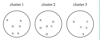
如图认为x代表一类文档,o代表一类文档,方框代表一类文档,完美的聚类显然是应该把各种不同的图形放入一类,事实上我们很难找到完美的聚类方法,各种方法在实际中难免有偏差,所以我们才需要对聚类算法进行评价看我们采用的方法是不是好的算法。
(1) purity评价法:
purity方法是极为简单的一种聚类评价方法,只需计算正确聚类的文档数占总文档数的比例:
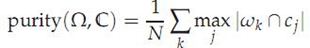
其中Ω = {ω1,ω2, . . . ,ωK}是聚类的集合ωK表示第k个聚类的集合。C = {c1, c2, . . . , cJ}是文档集合,cJ表示第J个文档。N表示文档总数。
如上图的purity = ( 3+ 4 + 5) / 17 = 0.71
其中第一类正确的有5个,第二个4个,第三个3个,总文档数17。
purity方法的优势是方便计算,值在0~1之间,完全错误的聚类方法值为0,完全正确的方法值为1。同时,purity方法的缺点也很明显它无法对退化的聚类方法给出正确的评价,设想如果聚类算法把每篇文档单独聚成一类,那么算法认为所有文档都被正确分类,那么purity值为1!而这显然不是想要的结果。
(2) RI评价法:
实际上这是一种用排列组合原理来对聚类进行评价的手段,公式如下:
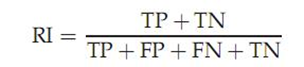
其中TP是指被聚在一类的两个文档被正确分类了,TN是只不应该被聚在一类的两个文档被正确分开了,FP只不应该放在一类的文档被错误的放在了一类,FN指不应该分开的文档被错误的分开了。对上图

TP+FP = C(2,6) + C(2,6) + C(2,5) = 15 + 15 + 10 = 40
其中C(n,m)是指在m中任选n个的组合数。
TP = C(2,5) + C(2,4) + C(2,3) + C(2,2) = 20
FP = 40 - 20 = 20
同理:
TN+FN= C(1,6) * C(1,6)+ C(1,6)* C(1,5) + C(1,6)* C(1,5)=96
FN= C(1,5) * C(1,3)+ C(1,1)* C(1,4) + C(1,1)* C(1,3)+ C(1,1)* C(1,2)=24
TN=96-24=72
所以RI = ( 20 + 72) / ( 20 + 20 + 72 +24) = 0.68
(三):F值评价法
这是基于上述RI方法衍生出的一个方法,
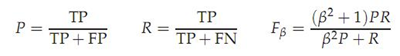
注:p是查全率,R是查准率,当β>1时查全率更有影响,当β<1时查准率更有影响,当β=1时退化为标准的F1,详细查阅机器学习P30
RI方法有个特点就是把准确率和召回率看得同等重要,事实上有时候我们可能需要某一特性更多一点,这时候就适合F值方法
Precision=TP/(TP+FP)
Recall=TP/(TP+FN)
F1=2×Recall×Precision/(Recall+Precision)
Precision=20/40=0.5
Recall=20/44=0.455
F1=(2*0.5*0.455)/(0.5+0.455)=0.48
四、聚类分析结果的降维可视化—TSNE
我们总喜欢能够直观地展示研究结果,聚类也不例外。然而,通常来说输入的特征数是高维的(大于3维),一般难以直接以原特征对聚类结果进行展示。而TSNE提供了一种有效的数据降维方式,让我们可以在2维或者3维的空间中展示聚类结果。
2.k-medoids(k中心点)
kmeans这种方法虽然快速高效,是大规模数据聚类分析中首选的方法,但是它也有一些短板,比如在数据集中有脏数据时,由于其对每一个类的准则函数为平方误差,当样本数据中出现了不合理的极端值,会导致最终聚类结果产生一定的误差,而本篇将要介绍的K-medoids(中心点)聚类法在削弱异常值的影响上就有着其过人之处。
与K-means算法类似,区别在于中心点的选取,K-means中选取的中心点为当前类中所有点的重心,而K-medoids法选取的中心点为当前cluster中存在的一点,准则函数是当前cluster中所有其他点到该中心点的距离之和最小,这就在一定程度上削弱了异常值的影响,但缺点是计算较为复杂,耗费的计算机时间比K-means多。
具体的算法流程如下:
1.在总体n个样本点中任意选取k个点作为medoids
2.按照与medoids最近的原则,将剩余的n-k个点分配到当前最佳的medoids代表的类中
3.对于第i个类中除对应medoids点外的所有其他点,按顺序计算当其为新的medoids时,准则函数的值,遍历所有可能,选取准则函数最小时对应的点作为新的medoids
4.重复2-3的过程,直到所有的medoids点不再发生变化或已达到设定的最大迭代次数
5.产出最终确定的k个类
在Python中关于K-medoids的第三方算法实在是够冷门,经过笔者一番查找,终于在一个久无人维护的第三方模块pyclust中找到了对应的方法KMedoids(),若要对制定的数据进行聚类,使用格式如下:
KMedoids(n_clusters=n).fit_predict(data),其中data即为将要预测的样本集,下面以具体示例进行展示
from pyclust import KMedoids
import numpy as np
from sklearn.manifold import TSNE
import matplotlib.pyplot as plt

'''构造示例数据集(加入少量脏数据)'''
data1 = np.random.normal(0,0.9,(1000,10))
data2 = np.random.normal(1,0.9,(1000,10))
data3 = np.random.normal(2,0.9,(1000,10))
data4 = np.random.normal(3,0.9,(1000,10))
data5 = np.random.normal(50,0.9,(50,10))

data = np.concatenate((data1,data2,data3,data4,data5))

'''准备可视化需要的降维数据'''
data_TSNE = TSNE(learning_rate=100).fit_transform(data)

'''对不同的k进行试探性K-medoids聚类并可视化'''
plt.figure(figsize=(12,8))
for i in range(2,6):
    k = KMedoids(n_clusters=i,distance='euclidean',max_iter=1000).fit_predict(data)
    colors = ([['red','blue','black','yellow','green'][i] for i in k])
    plt.subplot(219+i)
    plt.scatter(data_TSNE[:,0],data_TSNE[:,1],c=colors,s=10)
    plt.title('K-medoids Resul of '.format(str(i)))
由于pyclust长久未被维护,可以参考这个:
https://www.jianshu.com/p/c0fada830a35
三种聚类总体的介绍可以看简书这篇文章
https://www.jianshu.com/p/841ecdaab847
reference: