基于MNIST手写数字数据集的数字识别小程序（CNN改进版）

上次的程序识别率只能达到91%左右，所以没什么乱用，今天使用CNN模型进行改进，识别率能达到98%。

上码！

 1 import tensorflow as tf
 2 import tensorflow.examples.tutorials.mnist.input_data as input_data
 3 mnist = input_data.read_data_sets('/temp/', one_hot=True)
 4 
 5 
 6 #定义两个函数用于初始化
 7 #避免0梯度
 8 def weight_variable(shape):
 9     initial = tf.truncated_normal(shape,stddev=0.1)
10     return tf.Variable(initial)
11 
12 def bias_variable(shape):
13     initial = tf.constant(0.1,shape=shape)
14     return tf.Variable(initial)
15 
16 #卷积和池化
17 def conv2d(x,W):
18     return tf.nn.conv2d(x,W,strides=[1,1,1,1],padding='SAME')
19 
20 def max_pool_2x2(x):
21     return tf.nn.max_pool(x,ksize=[1,2,2,1],strides=[1,2,2,1],padding='SAME')
22 
23 #输入和输出
24 x = tf.placeholder(tf.float32,[None,784])
25 y_ = tf.placeholder(tf.float32,[None,10])
26 
27 #tensorflow 对话
28 sess = tf.Session()
29 
30 #设置第一层卷积
31 W_conv1 = weight_variable([5,5,1,32])
32 b_conv1 = bias_variable([32])
33 
34 x_image = tf.reshape(x,[-1,28,28,1])
35 
36 h_conv1 = tf.nn.relu(conv2d(x_image,W_conv1)+b_conv1)
37 h_pool1 = max_pool_2x2(h_conv1)
38 
39 #第二层卷积
40 W_conv2 = weight_variable([5,5,32,64])
41 b_conv2 = bias_variable([64])
42 
43 h_conv2 = tf.nn.relu(conv2d(h_pool1,W_conv2)+b_conv2)
44 h_pool2 = max_pool_2x2(h_conv2)
45 
46 #密集连接层  全连接层
47 W_fc1 = weight_variable([7*7*64,1024])
48 b_fc1 = bias_variable([1024])
49 
50 h_pool2_flat = tf.reshape(h_pool2,[-1,7*7*64])
51 h_fc1 = tf.nn.relu(tf.matmul(h_pool2_flat,W_fc1)+b_fc1)
52 
53 #减少过拟合 加入dropout
54 keep_prob = tf.placeholder("float")
55 h_fc1_drop = tf.nn.dropout(h_fc1,keep_prob)
56 
57 #输出层
58 W_fc2 = weight_variable([1024,10])
59 b_fc2 = bias_variable([10])
60 
61 y_conv = tf.nn.softmax(tf.matmul(h_fc1_drop,W_fc2)+b_fc2)
62 
63 #交叉熵
64 cross_entropy = -tf.reduce_sum(y_*tf.log(y_conv))
65 train_step = tf.train.AdamOptimizer(1e-4).minimize(cross_entropy)
66 
67 #评估模型
68 correct_prediction = tf.equal(tf.argmax(y_conv,1),tf.argmax(y_,1))
69 accuracy = tf.reduce_mean(tf.cast(correct_prediction,"float"))
70 sess.run(tf.initialize_all_variables())
71 
72 for i in range(2000):
73     batch = mnist.train.next_batch(50)
74     if i % 100 ==0:
75         train_accuracy = accuracy.eval(session=sess,feed_dict={x:batch[0],y_:batch[1],keep_prob:1.0})
76         print("step %d,training accuracy %g" %(i,train_accuracy))
77     train_step.run(session=sess,feed_dict={x:batch[0],y_:batch[1],keep_prob : 0.5})
78 
79 print ("test accuracy %g"%accuracy.eval(session=sess,feed_dict={x: mnist.test.images, y_: mnist.test.labels, keep_prob: 1.0}))

--------------------------------------------------------------华丽的分割线------------------------------------------------------------------------------

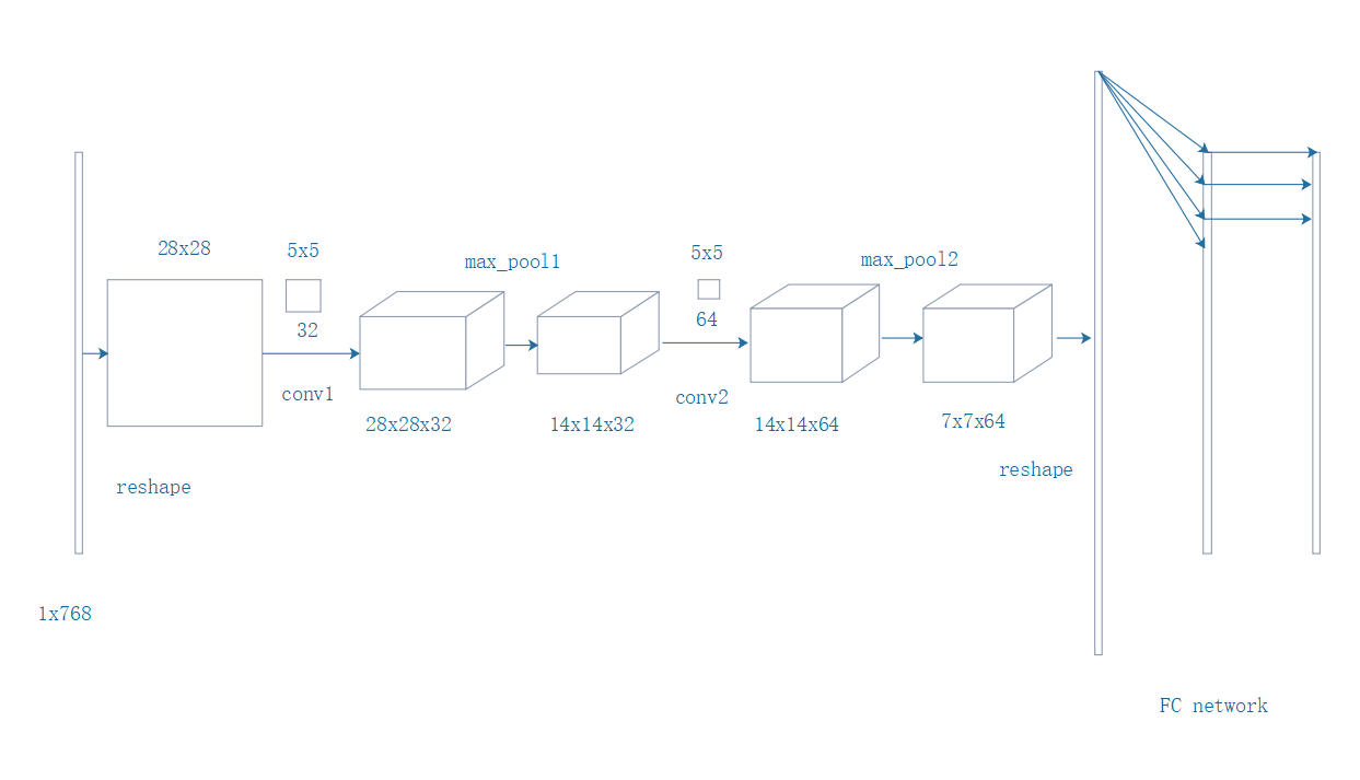
79行，比上次复杂了一点而已i，下面有一张图可以更好的帮助理解CNN网络。

首先是1~3行，这个就不解释了，不懂可以参考上一篇文章。

 6 #定义两个函数用于初始化
 7 #避免0梯度
 8 def weight_variable(shape):
 9     initial = tf.truncated_normal(shape,stddev=0.1)
10     return tf.Variable(initial)
11 
12 def bias_variable(shape):
13     initial = tf.constant(0.1,shape=shape)
14     return tf.Variable(initial)


6~14行是用于增加网络的层数，每增加一层就可以条用这两个函数来设置权重变量和偏置变量。
这里用到的tensorflow函数有：

tf.truncated_normal(shape, mean, stddev)   产生正太分布的函数，参数分别是张量维度、均值、方差　

tf.constant　　　　　　　　tensorflow的常量类型

tf.Variable　　　　　　　　tensorflow的变量类型


--------------------------------------------------------------华丽的分割线------------------------------------------------------------------------------

16 #卷积和池化
17 def conv2d(x,W):
18     return tf.nn.conv2d(x,W,strides=[1,1,1,1],padding='SAME')
19 
20 def max_pool_2x2(x):
21     return tf.nn.max_pool(x,ksize=[1,2,2,1],strides=[1,2,2,1],padding='SAME')

16~21行是定义卷积和池化，这里用到的tensorflow函数有：

 tf.nn.conv2d(input, filter, strides, padding) 　　　　 实现二维的卷积

 tf.nn.max_pool(value, ksize, strides, padding)       实现最大值池化操作

  W是卷积核，步长为1

 池化是[[1,2][2,1]]的矩阵，步长为2

--------------------------------------------------------------华丽的分割线------------------------------------------------------------------------------

23 #输入和输出
24 x = tf.placeholder(tf.float32,[None,784])
25 y_ = tf.placeholder(tf.float32,[None,10])
26 
27 #tensorflow 对话
28 sess = tf.Session()

23~28行就是我们的输入和真值的占位符设置，此外还有tensorflow的Session对话。

--------------------------------------------------------------华丽的分割线------------------------------------------------------------------------------

   前面定义了几个重要的函数，现在就开始构建我们的计算图了，先看图：

 

30 #设置第一层卷积
31 W_conv1 = weight_variable([5,5,1,32])
32 b_conv1 = bias_variable([32])
33 
34 x_image = tf.reshape(x,[-1,28,28,1])
35 
36 h_conv1 = tf.nn.relu(conv2d(x_image,W_conv1)+b_conv1)
37 h_pool1 = max_pool_2x2(h_conv1)


34行就是先把表示图片的1x768向量转化成矩阵形式，即转化为28x28形状，参数1表示单通道；
然后定31、32行设置我们的卷积核，大小是5x5的卷积核，输入通道数为1，输出通道数为32，偏置的个数也32个；
接着就是隐藏层的输出，这里使用的是RELU激活函数，也就是tensorflow的

tf.nn.relu 函数 ，参数就是我们的卷积函数加上偏置就得到隐藏层的输出；
最后是池化层的输出，这里用的卷积形式都是padding = ‘SAME' 形式，也就是输出形状宽(高)=输入形状宽(高)/步长
如图所示，得到我们的28x28x32和14x14x32的32卷积层和池化层

39 #第二层卷积
40 W_conv2 = weight_variable([5,5,32,64])
41 b_conv2 = bias_variable([64])
42 
43 h_conv2 = tf.nn.relu(conv2d(h_pool1,W_conv2)+b_conv2)
44 h_pool2 = max_pool_2x2(h_conv2)

根据图所示，构建第二层卷积层和池化层，这里不赘述了，参考第一层。

46 #密集连接层  全连接层
47 W_fc1 = weight_variable([7*7*64,1024])
48 b_fc1 = bias_variable([1024])
49 
50 h_pool2_flat = tf.reshape(h_pool2,[-1,7*7*64])
51 h_fc1 = tf.nn.relu(tf.matmul(h_pool2_flat,W_fc1)+b_fc1)

前面通过两层卷积和池化之后，需要重新转换为向量形式，作为全连接层的输入 也就是50行代码所示，
还有权重和偏置的设置如47、48行，这个和上一篇文章是一样的，理解了上一篇文章，然后根据图示，自然很容易理解了
最后的激活函数仍是使用RELU函数，到此计算图构建完毕。

--------------------------------------------------------------华丽的分割线------------------------------------------------------------------------------

53 #减少过拟合 加入dropout
54 keep_prob = tf.placeholder("float")
55 h_fc1_drop = tf.nn.dropout(h_fc1,keep_prob)
56 
57 #输出层
58 W_fc2 = weight_variable([1024,10])
59 b_fc2 = bias_variable([10])
60 
61 y_conv = tf.nn.softmax(tf.matmul(h_fc1_drop,W_fc2)+b_fc2)
62 
63 #交叉熵
64 cross_entropy = -tf.reduce_sum(y_*tf.log(y_conv))
65 train_step = tf.train.AdamOptimizer(1e-4).minimize(cross_entropy)

58~65行基本上是上一篇文章的内容，这里主要是53~55行，通过tensorflow的dropout来减少过拟合
原理大致是通过选择概率，随机使某些隐层神经元不工作，处于无法激活状态，在进行训练的多次迭代过程中
相当于产生多种不同的网络，最后输出的结果相当于这些网络的平均效果，以此达到减少过拟合。
与上一篇文章一样的，使用交叉熵作为损失函数，同时这里用新的优化算法Adam。

--------------------------------------------------------------华丽的分割线------------------------------------------------------------------------------

67 #评估模型
68 correct_prediction = tf.equal(tf.argmax(y_conv,1),tf.argmax(y_,1))
69 accuracy = tf.reduce_mean(tf.cast(correct_prediction,"float"))
70 sess.run(tf.initialize_all_variables())
71 
72 for i in range(2000):
73     batch = mnist.train.next_batch(50)
74     if i % 100 ==0:
75         train_accuracy = accuracy.eval(session=sess,feed_dict={x:batch[0],y_:batch[1],keep_prob:1.0})
76         print("step %d,training accuracy %g" %(i,train_accuracy))
77     train_step.run(session=sess,feed_dict={x:batch[0],y_:batch[1],keep_prob : 0.5})
78 
79 print ("test accuracy %g"%accuracy.eval(session=sess,feed_dict={x: mnist.test.images, y_: mnist.test.labels, keep_prob: 1.0}))

最后就是我们的评估模型了，别忘记了70行的我们需要对所有变量进行初始化。
然后就是训练我们的模型，每100次迭代输出一次测试结果，每次训练小批量数据50个，注意到keep_prob参数
该参数就是dropout所确定的概率，1.0就是全部神经元工作，0.5就是随机选择一半神经元不工作，以此达到减少过拟合。

代码就79行，下面来看看运行的结果：


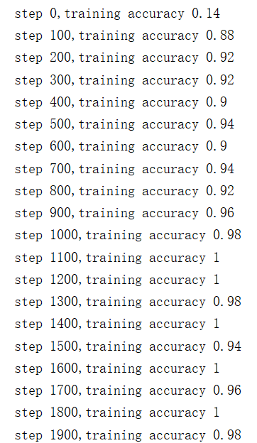
从精确率看来，平均水平能达到98%，从而改进了上一篇文章中的简单模型，
把准确率大幅提高，这样的网络才有较好的用途。
（但是还有更多其他的模型，仍然继续深入大坑！）