下面是我从cs231n上整理的神经网络的入门实现,麻雀虽小,五脏俱全,基本上神经网络涉及到的知识点都有在代码中体现。
理论看上千万遍,不如看一遍源码跑一跑。
源码上我已经加了很多注释,结合代码看一遍很容易理解。
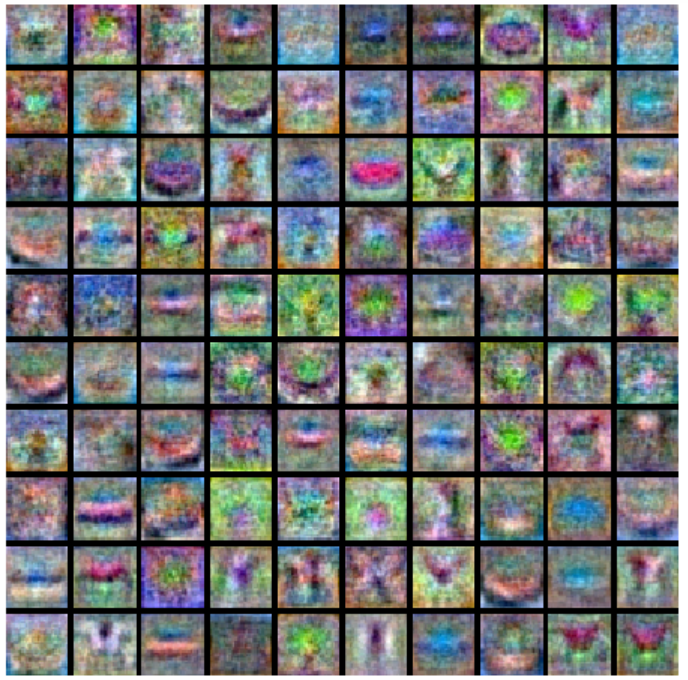
最后可视化权重的图:
主文件,用来训练调参
two_layer_net.py


  1 # coding: utf-8
  2
  3 # 实现一个简单的神经网络并在CIFAR10上测试性能
  4
  5 import numpy as np
  6 import matplotlib.pyplot as plt
  7 from neural_net import TwoLayerNet
  8 from data_utils import load_CIFAR10
  9 from vis_utils import visualize_grid
 10
 11 def get_CIFAR10_data(num_training=49000, num_validation=1000, num_test=1000):
 12     cifar10_dir = 'cs231n/datasets/cifar-10-batches-py'
 13     X_train, y_train, X_test, y_test = load_CIFAR10(cifar10_dir)
 14
 15     # 采样
 16     mask = list(range(num_training, num_training + num_validation))
 17     X_val = X_train[mask]
 18     y_val = y_train[mask]
 19     mask = list(range(num_training))
 20     X_train = X_train[mask]
 21     y_train = y_train[mask]
 22     mask = list(range(num_test))
 23     X_test = X_test[mask]
 24     y_test = y_test[mask]
 25
 26     # 归一化操作:减去均值,使得数据以0为中心
 27     mean_image = np.mean(X_train, axis=0)
 28     X_train -= mean_image
 29     X_val -= mean_image
 30     X_test -= mean_image
 31
 32     X_train = X_train.reshape(num_training, -1)
 33     X_val = X_val.reshape(num_validation, -1)
 34     X_test = X_test.reshape(num_test, -1)
 35
 36     return X_train, y_train, X_val, y_val, X_test, y_test
 37
 38
 39 X_train, y_train, X_val, y_val, X_test, y_test = get_CIFAR10_data()
 40 print('Train data shape: ', X_train.shape)
 41 print('Train labels shape: ', y_train.shape)
 42 print('Validation data shape: ', X_val.shape)
 43 print('Validation labels shape: ', y_val.shape)
 44 print('Test data shape: ', X_test.shape)
 45 print('Test labels shape: ', y_test.shape)
 46
 47
 48 #第一次训练
 49 input_size = 32 * 32 * 3
 50 hidden_size = 50
 51 num_classes = 10
 52 net = TwoLayerNet(input_size, hidden_size, num_classes)
 53 stats = net.train(X_train, y_train, X_val, y_val,
 54             num_iters=1000, batch_size=200,
 55             learning_rate=1e-4, learning_rate_decay=0.95,
 56             reg=0.25, verbose=True)
 57 val_acc = (net.predict(X_val) == y_val).mean()
 58 print('Validation accuracy: ', val_acc)
 59
 60 #效果不太理想,debug
 61
 62 # 先画一下loss和正确率的曲线看一看
 63 plt.subplot(2, 1, 1)
 64 plt.plot(stats['loss_history'])
 65 plt.title('Loss history')
 66 plt.xlabel('Iteration')
 67 plt.ylabel('Loss')
 68
 69 plt.subplot(2, 1, 2)
 70 plt.plot(stats['train_acc_history'], label='train')
 71 plt.plot(stats['val_acc_history'], label='val')
 72 plt.title('Classification accuracy history')
 73 plt.xlabel('Epoch')
 74 plt.ylabel('Clasification accuracy')
 75 plt.show()
 76
 77
 78
 79 #可视化一下权重
 80 def show_net_weights(net):
 81     W1 = net.params['W1']
 82     W1 = W1.reshape(32, 32, 3, -1).transpose(3, 0, 1, 2)
 83     plt.imshow(visualize_grid(W1, padding=3).astype('uint8'))
 84     plt.gca().axis('off')
 85     plt.show()
 86
 87 show_net_weights(net)
 88
 89
 90 #通过上面的曲线我们可以看到基本上loss还在线性下降,表示我们的loss下降的还不够。
 91 #一方面,我们可以加大学习率使loss更加快速的下降,另一方面,也可以增加迭代的次数,让loss继续下降。
 92 #还有,在训练集和验证集上的正确率没有明显差距,表明网络的容量可能不够,可以尝试增加网络的复杂度使之拥有更强的表达能力。
 93
 94
 95
 96 #下面是我调出来的参数,实际上选了很久 ,在测试集上的正确率在55%左右
 97 hidden_size = 150#[50,70,100,130]
 98 learning_rates = 1e-3#np.array([0.5,1,1.5])*1e-3
 99 regularization_strengths = 0.2#[0.1,0.2,0.3]
100 best_net = None
101 results = {}
102 best_val_acc = 0
103
104
105 for hs in hidden_size:
106     for lr in learning_rates:
107         for reg in regularization_strengths:
108
109             net = TwoLayerNet(input_size, hs, num_classes)
110             # Train the network
111             stats = net.train(X_train, y_train, X_val, y_val,
112             num_iters=3000, batch_size=200,
113             learning_rate=lr, learning_rate_decay=0.95,
114             reg= reg, verbose=False)
115             val_acc = (net.predict(X_val) == y_val).mean()
116             if val_acc > best_val_acc:
117                 best_val_acc = val_acc
118                 best_net = net
119             results[(hs,lr,reg)] = val_acc
120
121             plt.subplot(2, 1, 1)
122             plt.plot(stats['loss_history'])
123             plt.title('Loss history')
124             plt.xlabel('Iteration')
125             plt.ylabel('Loss')
126
127             plt.subplot(2, 1, 2)
128             plt.plot(stats['train_acc_history'], label='train')
129             plt.plot(stats['val_acc_history'], label='val')
130             plt.title('Classification accuracy history')
131             plt.xlabel('Epoch')
132             plt.ylabel('Clasification accuracy')
133             plt.show()
134
135
136 for hs,lr, reg in sorted(results):
137     val_acc = results[(hs, lr, reg)]
138     print ('hs %d lr %e reg %e val accuracy: %f' % (hs, lr, reg,  val_acc))
139
140 print ('best validation accuracy achieved during cross-validation: %f' % best_val_acc)
141
142
143 show_net_weights(best_net)
144 test_acc = (best_net.predict(X_test) == y_test).mean()
145 print('Test accuracy: ', test_acc)
定义神经网络和前向反向计算、损失函数、自动训练的类
neural_net.py
  1 import numpy as np
  2 import matplotlib.pyplot as plt
  3
  4 class TwoLayerNet(object):
  5   """
  6   两层的全连接网络。使用sotfmax损失函数和L2正则,非线性函数采用Relu函数。
  7   网络结构:input - fully connected layer - ReLU - fully connected layer - softmax
  8   """
  9
 10   def __init__(self, input_size, hidden_size, output_size, std=1e-4):
 11     """
 12     初始化模型。
 13     初始化权重矩阵W和偏置b。这里b置为零,但是Alexnet论文中说采用Relu函数激活时b置为1可以更快的收敛。
 14     参数都保存在self.params字典中。
 15     键为:
 16     W1 (D, H)
 17     b1 (H,)
 18     W2 (H, C)
 19     b2 (C,)
 20     D,H,C分别表示输入数据的维度,隐藏层大小,输出类别的个数
 21     """
 22     self.params = {}
 23     self.params['W1'] = std * np.random.randn(input_size, hidden_size)
 24     self.params['b1'] = np.zeros(hidden_size)
 25     self.params['W2'] = std * np.random.randn(hidden_size, output_size)
 26     self.params['b2'] = np.zeros(output_size)
 27
 28   def loss(self, X, y=None, reg=0.0):
 29     """
 30     如果是在训练过程,计算损失和梯度,如果是在测试过程,返回最后一层的输入,即每个类的得分。
 31
 32     Inputs:
 33     - X (N, D).  X[i] 为一个训练样本。
 34     - y: 标签。如果为None则表示是在进行测试过程,否则是在进行训练过程。
 35     - reg: Regularization strength.
 36
 37     Returns:
 38     如果y=None,返回shape为(N, C)的矩阵,scores[i, c]表示输入i在c类上的得分。
 39
 40     如果y!=None, 返回一个tuple:
 41     - loss: 包括数据损失和正则损失两部分。
 42     - grads: 各个参数的梯度。
 43     """
 44
 45     W1, b1 = self.params['W1'], self.params['b1']
 46     W2, b2 = self.params['W2'], self.params['b2']
 47     N, D = X.shape
 48     C=b2.shape[0]
 49
 50     #forward pass
 51     h1=np.maximum(0,np.dot(X,W1)+b1)
 52     h2=np.dot(h1,W2)+b2
 53     scores=h2
 54
 55     if y is None:
 56       return scores
 57
 58     # 计算loss
 59     shift_scores=scores-np.max(scores,axis=1).reshape(-1,1)
 60     exp_scores=np.exp(shift_scores)
 61     softmax_out=exp_scores/np.sum(exp_scores,axis=1).reshape(-1,1)
 62     loss=np.sum(-np.log(softmax_out[range(N),y]))/N+reg * (np.sum(W1 * W1) + np.sum(W2 * W2))
 63     print(np.sum(-np.log(softmax_out[range(N),y]))/N,reg * (np.sum(W1 * W1) + np.sum(W2 * W2)))
 64
 65     # Backward pass: 计算梯度,梯度的计算就是链式求导的过程
 66     grads = {}
 67
 68     dscores = softmax_out.copy()
 69     dscores[range(N),y]-=1
 70     dscores /= N
 71
 72     grads['W2']=np.dot(h1.T,dscores)+2*reg*W2
 73     grads['b2']=np.sum(dscores,axis=0)
 74
 75     dh=np.dot(dscores,W2.T)
 76     d_max=(h1>0)*dh
 77
 78     grads['W1'] = X.T.dot(d_max) + 2*reg * W1
 79     grads['b1'] = np.sum(d_max, axis = 0)
 80
 81     return loss, grads
 82
 83   def train(self, X, y, X_val, y_val,
 84             learning_rate=1e-3, learning_rate_decay=0.95,
 85             reg=5e-6, num_iters=100,
 86             batch_size=200, verbose=False):
 87     """
 88     自动化训练过程。采用SGD优化。
 89
 90     Inputs:
 91     - X (N, D):训练输入。
 92     - y (N,) :标签。 y[i] = c 表示X[i]的类别下标是c。
 93     - X_val (N_val, D):验证集输入。
 94     - y_val (N_val,): 验证集标签。
 95     - learning_rate:
 96     - learning_rate_decay: 学习率的损失因子。
 97     - reg: regularization strength。
 98     - num_iters: 迭代次数。
 99     - batch_size: 每次迭代的数据批大小。.
100     - verbose: 是否显示训练进度。
101     """
102     num_train = X.shape[0]
103     iterations_per_epoch = max(num_train / batch_size, 1)
104
105     loss_history = []
106     train_acc_history = []
107     val_acc_history = []
108
109     for it in range(num_iters):
110       #随机选择一批数据
111       idx = np.random.choice(num_train, batch_size, replace=True)
112       X_batch = X[idx]
113       y_batch = y[idx]
114       # 计算损失和梯度
115       loss, grads = self.loss(X_batch, y=y_batch, reg=reg)
116       loss_history.append(loss)
117       #更新参数
118       self.params['W2'] += - learning_rate * grads['W2']
119       self.params['b2'] += - learning_rate * grads['b2']
120       self.params['W1'] += - learning_rate * grads['W1']
121       self.params['b1'] += - learning_rate * grads['b1']
122       #可视化进度
123       if verbose and it % 100 == 0:
124         print('iteration %d / %d: loss %f' % (it, num_iters, loss))
125
126       # 每个epoch保存一次数据记录
127       if it % iterations_per_epoch == 0:
128         train_acc = (self.predict(X_batch) == y_batch).mean()
129         val_acc = (self.predict(X_val) == y_val).mean()
130         train_acc_history.append(train_acc)
131         val_acc_history.append(val_acc)
132         #学习率衰减
133         learning_rate *= learning_rate_decay
134     return {
135       'loss_history': loss_history,
136       'train_acc_history': train_acc_history,
137       'val_acc_history': val_acc_history,
138     }
139
140   def predict(self, X):
141     """
142     使用训练好的参数预测输入的标签。
143
144     Inputs:
145     - X (N, D): 需要预测的输入。
146
147     Returns:
148     - y_pred (N,):每个输入的预测分类下标。
149     """
150
151     h = np.maximum(0, X.dot(self.params['W1']) + self.params['b1'])
152     scores = h.dot(self.params['W2']) + self.params['b2']
153     y_pred = np.argmax(scores, axis=1)
154
155     return y_pred
载入CIFAR10数据的函数
data_utils.py
 1 from six.moves import cPickle as pickle
 2 import numpy as np
 3 import os
 4 from scipy.misc import imread
 5 import platform
 6
 7 def load_pickle(f):
 8     version = platform.python_version_tuple()
 9     if version[0] == '2':
10         return  pickle.load(f)
11     elif version[0] == '3':
12         return  pickle.load(f, encoding='latin1')
13     raise ValueError("invalid python version: {}".format(version))
14
15 def load_CIFAR_batch(filename):
16   """ CIRAR的数据是分批的,这个函数的功能是载入一批数据 """
17   with open(filename, 'rb') as f:
18     datadict = load_pickle(f) #以二进制方式打开文件
19     X = datadict['data']
20     Y = datadict['labels']
21     X = X.reshape(10000, 3, 32, 32).transpose(0,2,3,1).astype("float")
22     Y = np.array(Y)
23     return X, Y
24
25 def load_CIFAR10(ROOT):
26   """ load 所有的数据 """
27   xs = []
28   ys = []
29   for b in range(1,6):
30     f = os.path.join(ROOT, 'data_batch_%d' % (b, ))
31     X, Y = load_CIFAR_batch(f)
32     xs.append(X)
33     ys.append(Y)
34   Xtr = np.concatenate(xs)
35   Ytr = np.concatenate(ys)
36   del X, Y
37   Xte, Yte = load_CIFAR_batch(os.path.join(ROOT, 'test_batch'))
38   return Xtr, Ytr, Xte, Yte
可视化用到的函数
vis_utils.py
 1 from math import sqrt, ceil
 2 import numpy as np
 3
 4 def visualize_grid(Xs, ubound=255.0, padding=1):
 5   """
 6   #把4维的数据显示在平面图上,也就是把(N, H, W, C)N张3通道的图片同时显示出来
 7
 8   Inputs:
 9   - Xs:(N, H, W, C)shape的数据
10   - ubound: 像素会被放缩到【0,ubound】之间
11   - padding: 方块之间的间隔填充
12   """
13   (N, H, W, C) = Xs.shape
14   grid_size = int(ceil(sqrt(N)))
15   grid_height = H * grid_size + padding * (grid_size - 1)
16   grid_width = W * grid_size + padding * (grid_size - 1)
17   grid = np.zeros((grid_height, grid_width, C))
18   next_idx = 0
19   y0, y1 = 0, H
20   for y in range(grid_size):
21     x0, x1 = 0, W
22     for x in range(grid_size):
23       if next_idx < N:
24         img = Xs[next_idx]
25         low, high = np.min(img), np.max(img)
26         grid[y0:y1, x0:x1] = ubound * (img - low) / (high - low)
27         next_idx += 1
28       x0 += W + padding
29       x1 += W + padding
30     y0 += H + padding
31     y1 += H + padding
32   return grid