1.1 Deciding what to try next

当你调试你的学习算法时，当面对测试集你的算法效果不佳时，你会怎么做呢？
这里写图片描述

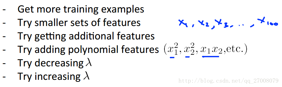
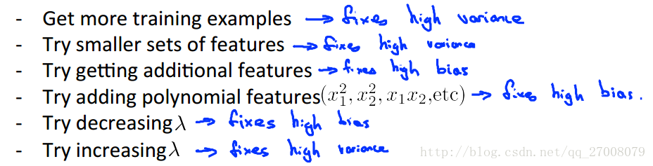
获得更多的训练样本？
尝试更少的特征？
尝试获取附加的特征？
尝试增加多项式的特征？
尝试增加 $\lambda$ ?
尝试减小 $\lambda$ ?

由此我们引出了机器学习诊疗法

1.2 EvaluaDng a hypothesis

这里写图片描述
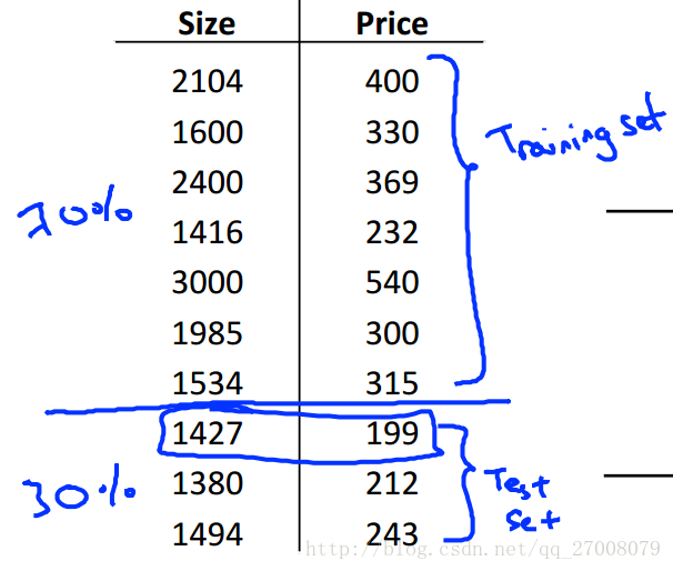
我们通过将数据集分成训练集和测试集，
将训练集训练出的参数用测试集数据测试性能。

线性回归时：
$J_{test}(\theta) = \frac{1}{2m_{test}}\sum_{i=1}^{m_{test}}(h_\theta(x^{(i)}_{test}) - y^{(i)}_{test}) ^ 2$

逻辑回归时：
$J_{test}(\theta) = -\frac{1}{2m_{test}}\sum_{i=1}^{m_{test}}y^{(i)}_{test}log(h_{\theta}(x^{(i)}_{test})) + (1-y^{(i)}_{test})log(1-h_{\theta}(x^{(i)}_{test}))$

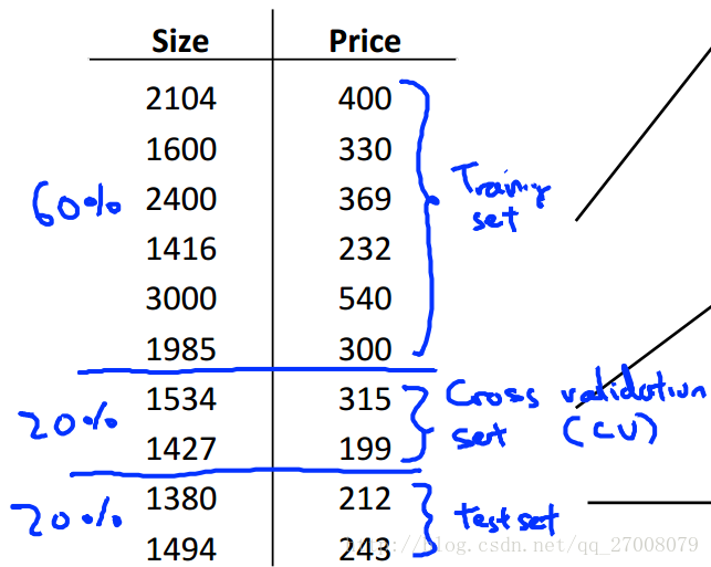
1.3 Model selecDon and training/validaDon/test sets

在多项式回归时，我们该怎么选择次数作为我们的假设模型呢？
这里写图片描述
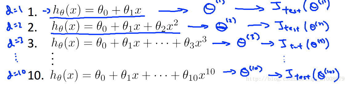
我们可以把数据集分为三类，训练集，交叉验证集和测试集，
用交叉验证集来作为评判选择的标准，选择合适的模型，而测试集则是作为算法性能的评判。

1.4 Diagnosing bias vs variance

这里写图片描述
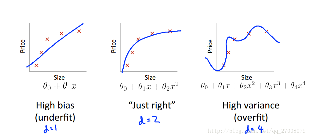
上面的图分别表示了高偏差，刚好，高方差

$J_{train}(\theta) = \frac{1}{2m_{train}}\sum_{i=1}^{m_{train}}(h_\theta(x^{(i)}_{train}) - y^{(i)}_{train}) ^ 2$
$J_{cv}(\theta) = \frac{1}{2m_{cv}}\sum_{i=1}^{m_{cv}}(h_\theta(x^{(i)}_{cv}) - y^{(i)}_{cv}) ^ 2$
这里写图片描述
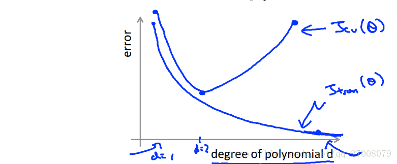
从图中可以看出，随着多项式次数的增大，训练集上的偏差逐渐变小，而交叉验证集上的偏差在减小到一定程度后开始升高。

在高偏差（欠拟合中）
$J_{train}(\theta)$ 很高
$J_{cv}(\theta) \approx J_{train}(\theta)$

在高方差（过拟合中）
$J_{train}(\theta)$ 很低
$J_{cv}(\theta) \gg J_{train}(\theta)$

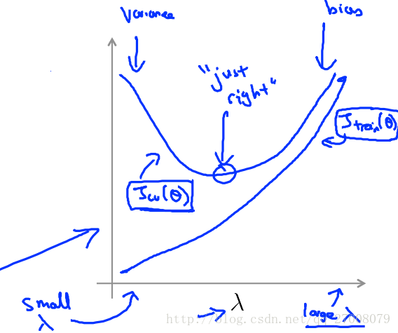
1.5 Regularization and bias/variance

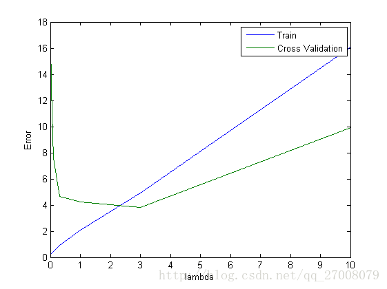
在加入正则化项后根据 $\lambda$ 的不同所得图如下
这里写图片描述

扫描二维码关注公众号，回复： 3480875 查看本文章

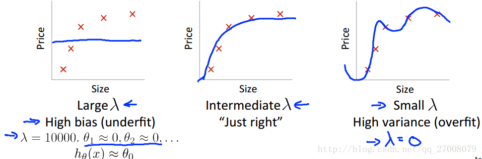
我们同样可以通过在交叉验证集上的测试选择较好的 $\lambda$ 值
这里写图片描述

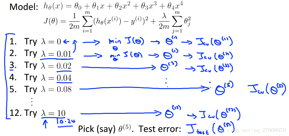
根据 $\lambda$ 大小画出的拟合曲线如下
这里写图片描述

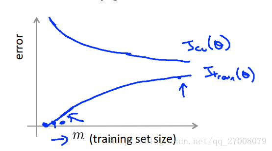
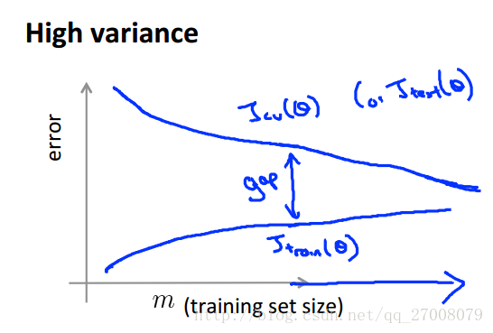
1.6 Learning curves

根据样本的大小与误差的关系我们可以画出一般的学习曲线模样
这里写图片描述

在高偏差的情况下，随着样本数目的增大，训练集上的误差和交叉验证集上的误差逐渐逼近。
这里写图片描述
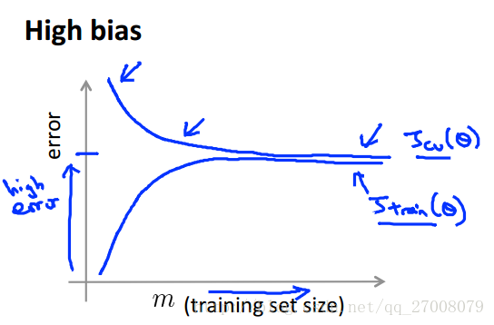
也就是说，增大样本的方法对高偏差的模型并不能起到一定作用

而模型处于高方差的情况下，增大样本可能会起到效果。
这里写图片描述

对开头提出的各种措施，我们看看他们适合于什么样的模型
这里写图片描述

2.1 Machine learning system design

以做一个垃圾邮件分类器为例。
我们需要寻找最频繁出现出现的n个单词（10000~50000）作为训练集，而不是随意手工寻找100个单词。

下面的做法帮助你改善你的模型。

收集大量的数据。 eg. “honeypot”项目。
从邮件信息中找寻复杂的特征（例如从邮件首部）。
从邮件体中找寻复杂的特征（discount 和discounts是否被对待一致，关于标点符号的特征）。
使用复杂的算法来检测邮件中的拼写错误。

对误差的分析

先开始一个简单算法使你能快速实现它，在你的交叉验证集上测试它。
画出学习曲线来判断是否更多的数据，更多的特征有助于改进算法。
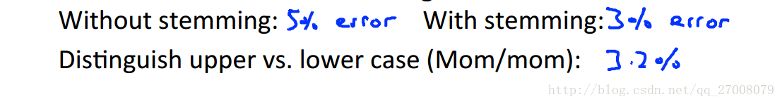
误差分析，在交叉验证集上检测你的算法，发现错误在某种类样本上出现的趋势。

将误差转变为一个单一的数值非常重要，否则很难判断我们所设计的学习算法的表现。
在误差分析中我们应使用定量计算来评判算法的表现。
这里写图片描述

2.2 Error metrics for skewed classes

以判断癌症的分类器为例。
建立逻辑回归模型 $h_\theta(x)$ ，y=1表示有癌症，y=0则没有。

假设你的算法在测试集上只有1%的错误，可实际上，测试集中只有0.5%的病人患有癌症，因此我们可以通过下面的方法来提高正确率。
这里写图片描述

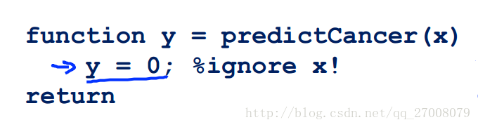
从上面的例子我们可以知道正确率不足以表现一个算法的优劣（在某些正例或反例及其少的数据集中），因此我们引入了Precision/Recall。

这里写图片描述
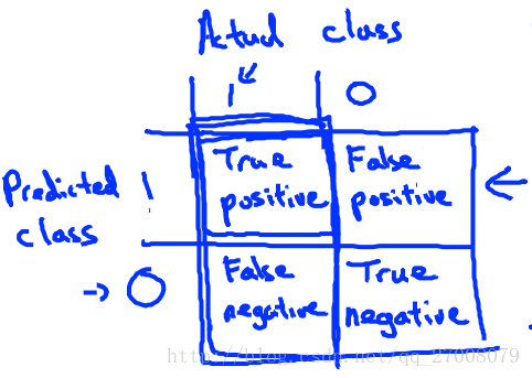
Precision（准确率）
在我们预测y=1的数据中，真正得癌症的比重。
$\frac{True　pos}{predicted　pos} = \frac{True　pos}{True　pos+ false　pos}$

Recal（召回率）
在真正得癌症的数据中，我们预测癌症所占的比重。
$\frac{True　pos}{actual　pos} = \frac{True　pos}{True　pos+ false　neg}$

在前面我们提到，将误差转变为一个单一的数值非常重要，因为这样我们才能方便的比较不同算法之间的优劣。现在我们有precision和recall两个衡量标准，我们需要权衡两者。如果用Logistic回归模型预测病人是否患癌症，考虑下面的情况：

假设考虑到一个正常人如果误判为癌症，将会承受不必要的心理和生理压力，所以我们要有很大把握才预测一个病人患癌症(y=1)。那么一种方式就是提高阙值(threshold)，不妨设我们将阙值提高到0.7，即：

Predict 1 if: hθ(x)≥0.7
Predict 0 if: hθ(x)<0.7

在这种情况下，我们将会有较高的precision，但是recall将会变低。

假设考虑到一个已经患癌症的病人如果误判为没有患癌症，那么病人可能将因不能及时治疗而失去宝贵生命，所以我们想要避免错过癌症患者的一种方式就是降低阙值，假设降低到0.3, 即

Predict 1 if: hθ(x)≥0.3
Predict 0 if: hθ(x)<0.3

在这种情况下，将得到较高的recall，但是precision将会下降。

为了将precision和Recal转变为一个单一数值，我们引入了

F=2PRP+R $F = 2\frac{PR}{P+R}$

3. 程序代码

在这次程序中，你首先进行了线性回归，然后画出了学习曲线，之后进行多项式回归，并画出学习曲线。最后比较了不同的 $\lambda$ 在训练集和交叉验证集上的效果。
ex5.m

%% Machine Learning Online Class
%  Exercise 5 | Regularized Linear Regression and Bias-Variance
%
%  Instructions
%  ------------
% 
%  This file contains code that helps you get started on the
%  exercise. You will need to complete the following functions:
%
%     linearRegCostFunction.m
%     learningCurve.m
%     validationCurve.m
%
%  For this exercise, you will not need to change any code in this file,
%  or any other files other than those mentioned above.
%

%% Initialization
clear ; close all; clc

%% =========== Part 1: Loading and Visualizing Data =============
%  We start the exercise by first loading and visualizing the dataset. 
%  The following code will load the dataset into your environment and plot
%  the data.
%

% Load Training Data
fprintf('Loading and Visualizing Data ...\n')

% Load from ex5data1: 
% You will have X, y, Xval, yval, Xtest, ytest in your environment
load ('ex5data1.mat');

% m = Number of examples
m = size(X, 1);

% Plot training data
plot(X, y, 'rx', 'MarkerSize', 10, 'LineWidth', 1.5);
xlabel('Change in water level (x)');
ylabel('Water flowing out of the dam (y)');

fprintf('Program paused. Press enter to continue.\n');
pause;

%% =========== Part 2: Regularized Linear Regression Cost =============
%  You should now implement the cost function for regularized linear 
%  regression. 
%

theta = [1 ; 1];
J = linearRegCostFunction([ones(m, 1) X], y, theta, 1);

fprintf(['Cost at theta = [1 ; 1]: %f '...
         '\n(this value should be about 303.993192)\n'], J);

fprintf('Program paused. Press enter to continue.\n');
pause;

%% =========== Part 3: Regularized Linear Regression Gradient =============
%  You should now implement the gradient for regularized linear 
%  regression.
%

theta = [1 ; 1];
[J, grad] = linearRegCostFunction([ones(m, 1) X], y, theta, 1);

fprintf(['Gradient at theta = [1 ; 1]:  [%f; %f] '...
         '\n(this value should be about [-15.303016; 598.250744])\n'], ...
         grad(1), grad(2));

fprintf('Program paused. Press enter to continue.\n');
pause;


%% =========== Part 4: Train Linear Regression =============
%  Once you have implemented the cost and gradient correctly, the
%  trainLinearReg function will use your cost function to train 
%  regularized linear regression.
% 
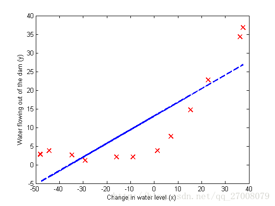
%  Write Up Note: The data is non-linear, so this will not give a great 
%                 fit.
%

%  Train linear regression with lambda = 0
lambda = 0;
[theta] = trainLinearReg([ones(m, 1) X], y, lambda);

%  Plot fit over the data
plot(X, y, 'rx', 'MarkerSize', 10, 'LineWidth', 1.5);
xlabel('Change in water level (x)');
ylabel('Water flowing out of the dam (y)');
hold on;
plot(X, [ones(m, 1) X]*theta, '--', 'LineWidth', 2)
hold off;

fprintf('Program paused. Press enter to continue.\n');
pause;


%% =========== Part 5: Learning Curve for Linear Regression =============
%  Next, you should implement the learningCurve function. 
%
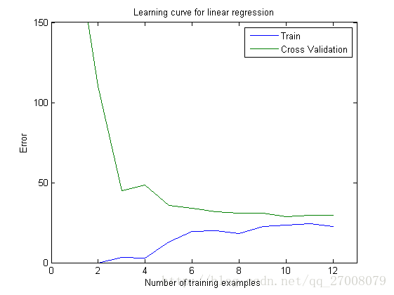
%  Write Up Note: Since the model is underfitting the data, we expect to
%                 see a graph with "high bias" -- Figure 3 in ex5.pdf 
%

lambda = 0;
[error_train, error_val] = ...
    learningCurve([ones(m, 1) X], y, ...
                  [ones(size(Xval, 1), 1) Xval], yval, ...
                  lambda);

plot(1:m, error_train, 1:m, error_val);
title('Learning curve for linear regression')
legend('Train', 'Cross Validation')
xlabel('Number of training examples')
ylabel('Error')
axis([0 13 0 150])

fprintf('# Training Examples\tTrain Error\tCross Validation Error\n');
for i = 1:m
    fprintf('  \t%d\t\t%f\t%f\n', i, error_train(i), error_val(i));
end

fprintf('Program paused. Press enter to continue.\n');
pause;

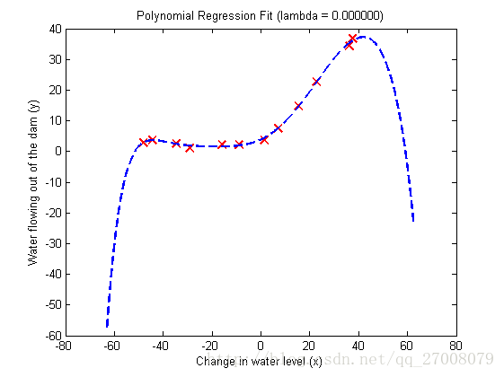
%% =========== Part 6: Feature Mapping for Polynomial Regression =============
%  One solution to this is to use polynomial regression. You should now
%  complete polyFeatures to map each example into its powers
%

p = 8;

% Map X onto Polynomial Features and Normalize
X_poly = polyFeatures(X, p);
[X_poly, mu, sigma] = featureNormalize(X_poly);  % Normalize
X_poly = [ones(m, 1), X_poly];                   % Add Ones

% Map X_poly_test and normalize (using mu and sigma)
X_poly_test = polyFeatures(Xtest, p);
X_poly_test = bsxfun(@minus, X_poly_test, mu);
X_poly_test = bsxfun(@rdivide, X_poly_test, sigma);
X_poly_test = [ones(size(X_poly_test, 1), 1), X_poly_test];         % Add Ones

% Map X_poly_val and normalize (using mu and sigma)
X_poly_val = polyFeatures(Xval, p);
X_poly_val = bsxfun(@minus, X_poly_val, mu);
X_poly_val = bsxfun(@rdivide, X_poly_val, sigma);
X_poly_val = [ones(size(X_poly_val, 1), 1), X_poly_val];           % Add Ones

fprintf('Normalized Training Example 1:\n');
fprintf('  %f  \n', X_poly(1, :));

fprintf('\nProgram paused. Press enter to continue.\n');
pause;



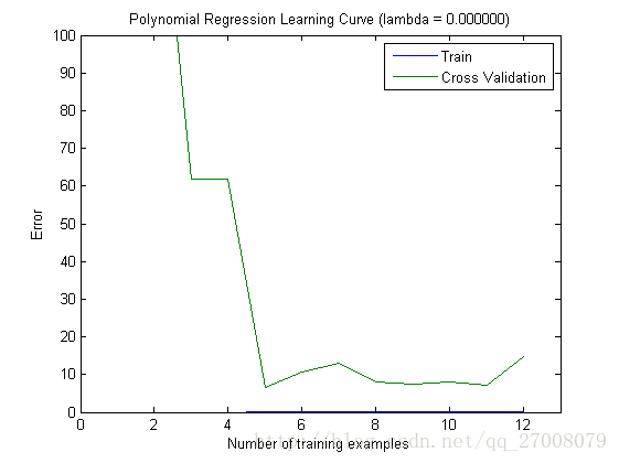
%% =========== Part 7: Learning Curve for Polynomial Regression =============
%  Now, you will get to experiment with polynomial regression with multiple
%  values of lambda. The code below runs polynomial regression with 
%  lambda = 0. You should try running the code with different values of
%  lambda to see how the fit and learning curve change.
%

lambda = 0;
[theta] = trainLinearReg(X_poly, y, lambda);

% Plot training data and fit
figure(1);
plot(X, y, 'rx', 'MarkerSize', 10, 'LineWidth', 1.5);
plotFit(min(X), max(X), mu, sigma, theta, p);
xlabel('Change in water level (x)');
ylabel('Water flowing out of the dam (y)');
title (sprintf('Polynomial Regression Fit (lambda = %f)', lambda));

figure(2);
[error_train, error_val] = ...
    learningCurve(X_poly, y, X_poly_val, yval, lambda);
plot(1:m, error_train, 1:m, error_val);

title(sprintf('Polynomial Regression Learning Curve (lambda = %f)', lambda));
xlabel('Number of training examples')
ylabel('Error')
axis([0 13 0 100])
legend('Train', 'Cross Validation')

fprintf('Polynomial Regression (lambda = %f)\n\n', lambda);
fprintf('# Training Examples\tTrain Error\tCross Validation Error\n');
for i = 1:m
    fprintf('  \t%d\t\t%f\t%f\n', i, error_train(i), error_val(i));
end

fprintf('Program paused. Press enter to continue.\n');
pause;

%% =========== Part 8: Validation for Selecting Lambda =============
%  You will now implement validationCurve to test various values of 
%  lambda on a validation set. You will then use this to select the
%  "best" lambda value.
%

[lambda_vec, error_train, error_val] = ...
    validationCurve(X_poly, y, X_poly_val, yval);

close all;
plot(lambda_vec, error_train, lambda_vec, error_val);
legend('Train', 'Cross Validation');
xlabel('lambda');
ylabel('Error');

fprintf('lambda\t\tTrain Error\tValidation Error\n');
for i = 1:length(lambda_vec)
    fprintf(' %f\t%f\t%f\n', ...
            lambda_vec(i), error_train(i), error_val(i));
end

fprintf('Program paused. Press enter to continue.\n');
pause;

linearRegCostFunction

function [J, grad] = linearRegCostFunction(X, y, theta, lambda)
%LINEARREGCOSTFUNCTION Compute cost and gradient for regularized linear 
%regression with multiple variables
%   [J, grad] = LINEARREGCOSTFUNCTION(X, y, theta, lambda) computes the 
%   cost of using theta as the parameter for linear regression to fit the 
%   data points in X and y. Returns the cost in J and the gradient in grad

% Initialize some useful values
m = length(y); % number of training examples

% You need to return the following variables correctly 
J = 0;
grad = zeros(size(theta));

% ====================== YOUR CODE HERE ======================
% Instructions: Compute the cost and gradient of regularized linear 
%               regression for a particular choice of theta.
%
%               You should set J to the cost and grad to the gradient.
%
J = 1/2/m* sum((X*theta - y) .^ 2) + lambda/2/m * sum(theta(2:end) .^ 2);

grad = 1/m* (X'*(X*theta - y));
grad(2:end) = grad(2:end) + lambda/m*theta(2:end);


% =========================================================================

grad = grad(:);

end

learningCurve.m

function [error_train, error_val] = ...
    learningCurve(X, y, Xval, yval, lambda)
%LEARNINGCURVE Generates the train and cross validation set errors needed 
%to plot a learning curve
%   [error_train, error_val] = ...
%       LEARNINGCURVE(X, y, Xval, yval, lambda) returns the train and
%       cross validation set errors for a learning curve. In particular, 
%       it returns two vectors of the same length - error_train and 
%       error_val. Then, error_train(i) contains the training error for
%       i examples (and similarly for error_val(i)).
%
%   In this function, you will compute the train and test errors for
%   dataset sizes from 1 up to m. In practice, when working with larger
%   datasets, you might want to do this in larger intervals.
%

% Number of training examples
m = size(X, 1);

% You need to return these values correctly
error_train = zeros(m, 1);
error_val   = zeros(m, 1);

% ====================== YOUR CODE HERE ======================
% Instructions: Fill in this function to return training errors in 
%               error_train and the cross validation errors in error_val. 
%               i.e., error_train(i) and 
%               error_val(i) should give you the errors
%               obtained after training on i examples.
%
% Note: You should evaluate the training error on the first i training
%       examples (i.e., X(1:i, :) and y(1:i)).
%
%       For the cross-validation error, you should instead evaluate on
%       the _entire_ cross validation set (Xval and yval).
%
% Note: If you are using your cost function (linearRegCostFunction)
%       to compute the training and cross validation error, you should 
%       call the function with the lambda argument set to 0. 
%       Do note that you will still need to use lambda when running
%       the training to obtain the theta parameters.
%
% Hint: You can loop over the examples with the following:
%
%       for i = 1:m
%           % Compute train/cross validation errors using training examples 
%           % X(1:i, :) and y(1:i), storing the result in 
%           % error_train(i) and error_val(i)
%           ....
%           
%       end
%

% ---------------------- Sample Solution ----------------------

for i=1:m
    theta = trainLinearReg(X(1:i, :), y(1:i), lambda);
    error_train(i) = linearRegCostFunction(X(1:i, :), y(1:i), theta, 0);
    error_val(i) = linearRegCostFunction(Xval, yval, theta, 0);
end


% -------------------------------------------------------------

% =========================================================================

end

validationCurve.m

function [lambda_vec, error_train, error_val] = ...
    validationCurve(X, y, Xval, yval)
%VALIDATIONCURVE Generate the train and validation errors needed to
%plot a validation curve that we can use to select lambda
%   [lambda_vec, error_train, error_val] = ...
%       VALIDATIONCURVE(X, y, Xval, yval) returns the train
%       and validation errors (in error_train, error_val)
%       for different values of lambda. You are given the training set (X,
%       y) and validation set (Xval, yval).
%

% Selected values of lambda (you should not change this)
lambda_vec = [0 0.001 0.003 0.01 0.03 0.1 0.3 1 3 10]';

% You need to return these variables correctly.
error_train = zeros(length(lambda_vec), 1);
error_val = zeros(length(lambda_vec), 1);

% ====================== YOUR CODE HERE ======================
% Instructions: Fill in this function to return training errors in 
%               error_train and the validation errors in error_val. The 
%               vector lambda_vec contains the different lambda parameters 
%               to use for each calculation of the errors, i.e, 
%               error_train(i), and error_val(i) should give 
%               you the errors obtained after training with 
%               lambda = lambda_vec(i)
%
% Note: You can loop over lambda_vec with the following:
%
%       for i = 1:length(lambda_vec)
%           lambda = lambda_vec(i);
%           % Compute train / val errors when training linear 
%           % regression with regularization parameter lambda
%           % You should store the result in error_train(i)
%           % and error_val(i)
%           ....
%           
%       end
%
%
for i=1:size(lambda_vec, 1)
    theta = trainLinearReg(X, y, lambda_vec(i));
    error_train(i) = linearRegCostFunction(X, y, theta, 0);
    error_val(i) = linearRegCostFunction(Xval, yval, theta, 0);
end


% =========================================================================

end