Neural Networks:Learning

上周的课程学习了神经网络正向传播算法，这周的课程主要在于神经网络的反向更新过程。

1.1 Cost function

我们先回忆一下逻辑回归的价值函数
$J(\theta) = \frac{1}{m}[\sum_{i=1}^{m}y^{(i)}log(h_\theta(x^{(i)})) + (1-y^{(i)})log(1-h_\theta(x^{(i)}))] + \frac{\lambda}{2m}\sum_{j=1}^{n}\theta_j^2$

在神经网络中
$h_\theta(x)\epsilon R^K$ 　　　 $(h_\theta(x))_i = i^{th}output$
$J(\theta) = -\frac{1}{m}[\sum_{i=1}^{m}\sum_{k=1}^{K}y^{(i)}_klog(h_\theta(x^{(i)}_k)) + (1-y_k^{(i)})log(1 - h_\theta(x_k^{(i)}))] + \frac{\lambda}{2m}\sum_{l=1}^{L-1}\sum_{i=1}^{s_l}\sum_{j=1}^{s_{l+1}}(\theta_{ji}^{(l)})^2$

1.2 Backpropagation algorithm

使用梯度下降法求解价值函数 $J(\theta)$ 的最小值
我们需要知道 $\frac{\partial }{\partial \theta^{(l)}_{ij}}J(\theta)$

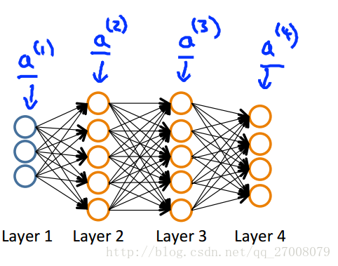
先给出一个样本(x, y)时的正向传播过程
这里写图片描述
$a^{(1)} = x$ 　　 $(add　a_0^{(1)})$
$z^{(2)} = \theta^{(1)}a^{(1)}$
$a^{(2)} = g(z^{(2)})$ 　　 $(add　a_0^{(2)})$
$z^{(3)} = \theta^{(2)}a^{(2)}$
$a^{(3)} = g(z^{(3)})$ 　　 $(add　a_0^{(3)})$
$z^{(4)} = \theta^{(3)}a^{(3)}$
$a^{(4)} = h_\theta(x) = g(z^{(4)})$

设置 $\delta^{(l)}_j$ 为第l层j节点的误差
$\delta^{(4)} = a^{(4)} - y$
$\delta^{(3)} = (\theta^{(3)})^{T}\delta^{(4)}.*g^{'}(z^{(3)})$
$\delta^{(2)} = (\theta^{(2)})^{T}\delta^{(3)}.*g^{'}(z^{(2)})$

算法步骤如下

Δ(l)ij=0 $\Delta^{(l)}_{ij} = 0$

for　k=1:m $for　k=1:m$
{

a(1)=x(k) $a^{(1)} = x^{(k)}$
按正向传播算法计算

a(l) $a^{(l)}$ 　　

l=2,3,4,⋯,L $l=2, 3, 4,\cdots,L$

δ(L)=a(L)−y $\delta^{(L)} = a^{(L)} - y$
按反向传播算法计算

δ(l) $\delta^{(l)}$ 　　

l=L−1,L−2,L−3,⋯,2 $l=L-1, L-2, L-3,\cdots,2$

Δ(l)=Δ(l)+δ(l+1)(a(l))T $\Delta^{(l)} = \Delta^{(l)} + \delta^{(l+1)}(a^{(l)})^T$ 　　

l=1,2,3,4,⋯,L−1 $l=1,2, 3, 4,\cdots,L-1$
}
别忘了加上正则化项。

∂∂θ(l)ijJ(θ)=D(l)ij=1mΔ(l)ij $\frac{\partial}{\partial \theta^{(l)}_{ij} }J(\theta) = D_{ij}^{(l)} = \frac{1}{m}\Delta^{(l)}_{ij}$ 　　　　　　　　　

j=0 $j=0$

∂∂θ(l)ijJ(θ)=D(l)ij=1mΔ(l)ij+λmθ(l)ij $\frac{\partial}{\partial \theta^{(l)}_{ij} }J(\theta) = D_{ij}^{(l)} = \frac{1}{m}\Delta^{(l)}_{ij} + \frac{\lambda}{m} \theta^{(l)}_{ij}$ 　　　　

j>=1 $j>=1$

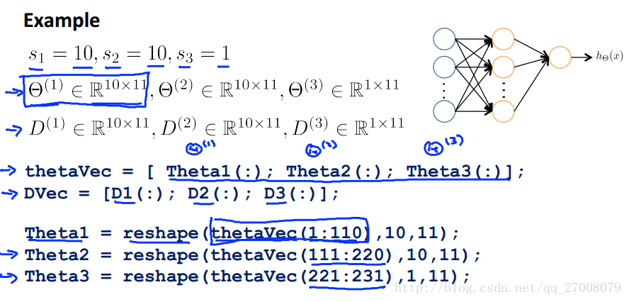
1.3 Unrolling parameters

这里写图片描述
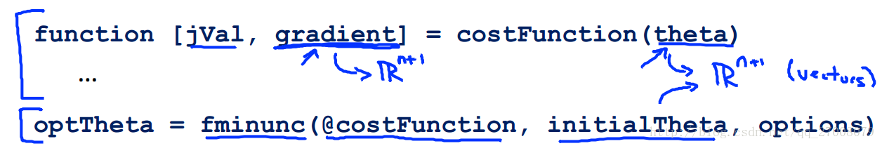
在上面的函数中，我们需要传递的参数为向量
而事实上，在我们上面的推理中可以发现 $\theta$ 和梯度都为矩阵形式，
所以我们需要把矩阵换为向量传递，在函数中将向量转换为矩阵使用。

下面举一个例子
这里写图片描述

1.4 Gradient checking

因为梯度计算方式的复杂，下面给出一种检测计算的方式。
我们学习过导数的几何意义如下。
这里写图片描述
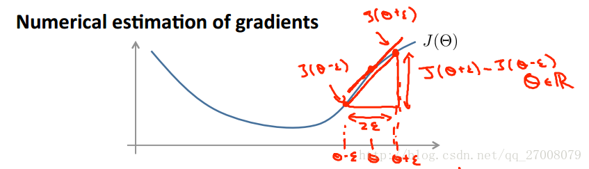
由此我们可以想到一种检测梯度的方式
$\theta = [\theta_1, \theta_2, \theta_3, \theta_4, \cdots, \theta_n]$
$\frac{\partial}{\partial \theta_1}J(\theta) \approx \frac{J(\theta_1 + \varepsilon, \theta_2, \theta_3, \cdots, \theta_n) - J(\theta_1 - \varepsilon, \theta_2, \theta_3, \cdots, \theta_n)}{2\varepsilon}$
$\frac{\partial}{\partial \theta_2}J(\theta) \approx \frac{J(\theta_1, \theta_2 + \varepsilon, \theta_3, \cdots, \theta_n) - J(\theta_1, \theta_2 - \varepsilon, \theta_3, \cdots, \theta_n)}{2\varepsilon}$
　 $\vdots$
$\frac{\partial}{\partial \theta_2}J(\theta) \approx \frac{J(\theta_1, \theta_2, \theta_3, \cdots, \theta_n + \varepsilon) - J(\theta_1, \theta_2, \theta_3, \cdots, \theta_n - \varepsilon)}{2\varepsilon}$

给出伪代码形式如下
这里写图片描述
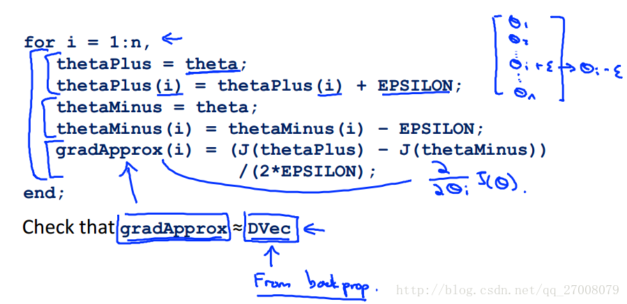
记住检测梯度的代码检测后要删去，不能用来训练数据集，会很慢。

1.5 Random initalization

在调用梯度下降法和先进的优化算法时，我们需要给出初始值
想一想，我们能和以往一样给初始值设为全0吗？

不行，根据正向传播算法，如果初始值都一样，则每层的单元值 $a^{(l)}_i$ 会相同
同样，根据反向传播算法，每个 $\delta^{(l)}_i$ 会相同

如此一来，每次更新后，输入到每层的各个单元值相同。

采用随机初始化
这里写图片描述
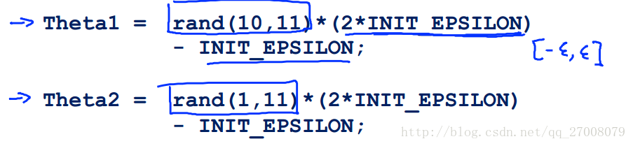
初始化 $\theta^{(l)}_{ij}$ 范围为 $[-\varepsilon, +\varepsilon]$

2. 程序代码

这次的程序和上周目的一致，都是手写数字识别，不过这周的代码要求自己训练出 $\theta$ 值

ex4.m

%% Machine Learning Online Class - Exercise 4 Neural Network Learning

%  Instructions
%  ------------
% 
%  This file contains code that helps you get started on the
%  linear exercise. You will need to complete the following functions 
%  in this exericse:
%
%     sigmoidGradient.m
%     randInitializeWeights.m
%     nnCostFunction.m
%
%  For this exercise, you will not need to change any code in this file,
%  or any other files other than those mentioned above.
%

%% Initialization
clear ; close all; clc

%% Setup the parameters you will use for this exercise
input_layer_size  = 400;  % 20x20 Input Images of Digits
hidden_layer_size = 25;   % 25 hidden units
num_labels = 10;          % 10 labels, from 1 to 10   
                          % (note that we have mapped "0" to label 10)

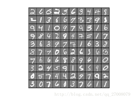
%% =========== Part 1: Loading and Visualizing Data =============
%  We start the exercise by first loading and visualizing the dataset. 
%  You will be working with a dataset that contains handwritten digits.
%

% Load Training Data
fprintf('Loading and Visualizing Data ...\n')

load('ex4data1.mat');
m = size(X, 1);

% Randomly select 100 data points to display
sel = randperm(size(X, 1));
sel = sel(1:100);

displayData(X(sel, :));

fprintf('Program paused. Press enter to continue.\n');
pause;


%% ================ Part 2: Loading Parameters ================
% In this part of the exercise, we load some pre-initialized 
% neural network parameters.

fprintf('\nLoading Saved Neural Network Parameters ...\n')

% Load the weights into variables Theta1 and Theta2
load('ex4weights.mat');

% Unroll parameters 
nn_params = [Theta1(:) ; Theta2(:)];

%% ================ Part 3: Compute Cost (Feedforward) ================
%  To the neural network, you should first start by implementing the
%  feedforward part of the neural network that returns the cost only. You
%  should complete the code in nnCostFunction.m to return cost. After
%  implementing the feedforward to compute the cost, you can verify that
%  your implementation is correct by verifying that you get the same cost
%  as us for the fixed debugging parameters.
%
%  We suggest implementing the feedforward cost *without* regularization
%  first so that it will be easier for you to debug. Later, in part 4, you
%  will get to implement the regularized cost.
%
fprintf('\nFeedforward Using Neural Network ...\n')

% Weight regularization parameter (we set this to 0 here).
lambda = 0;

J = nnCostFunction(nn_params, input_layer_size, hidden_layer_size, ...
                   num_labels, X, y, lambda);

fprintf(['Cost at parameters (loaded from ex4weights): %f '...
         '\n(this value should be about 0.287629)\n'], J);

fprintf('\nProgram paused. Press enter to continue.\n');
pause;

%% =============== Part 4: Implement Regularization ===============
%  Once your cost function implementation is correct, you should now
%  continue to implement the regularization with the cost.
%

fprintf('\nChecking Cost Function (w/ Regularization) ... \n')

% Weight regularization parameter (we set this to 1 here).
lambda = 1;

J = nnCostFunction(nn_params, input_layer_size, hidden_layer_size, ...
                   num_labels, X, y, lambda);

fprintf(['Cost at parameters (loaded from ex4weights): %f '...
         '\n(this value should be about 0.383770)\n'], J);

fprintf('Program paused. Press enter to continue.\n');
pause;


%% ================ Part 5: Sigmoid Gradient  ================
%  Before you start implementing the neural network, you will first
%  implement the gradient for the sigmoid function. You should complete the
%  code in the sigmoidGradient.m file.
%

fprintf('\nEvaluating sigmoid gradient...\n')

g = sigmoidGradient([-1 -0.5 0 0.5 1]);
fprintf('Sigmoid gradient evaluated at [-1 -0.5 0 0.5 1]:\n  ');
fprintf('%f ', g);
fprintf('\n\n');

fprintf('Program paused. Press enter to continue.\n');
pause;


%% ================ Part 6: Initializing Pameters ================
%  In this part of the exercise, you will be starting to implment a two
%  layer neural network that classifies digits. You will start by
%  implementing a function to initialize the weights of the neural network
%  (randInitializeWeights.m)

fprintf('\nInitializing Neural Network Parameters ...\n')

initial_Theta1 = randInitializeWeights(input_layer_size, hidden_layer_size);
initial_Theta2 = randInitializeWeights(hidden_layer_size, num_labels);

% Unroll parameters
initial_nn_params = [initial_Theta1(:) ; initial_Theta2(:)];


%% =============== Part 7: Implement Backpropagation ===============
%  Once your cost matches up with ours, you should proceed to implement the
%  backpropagation algorithm for the neural network. You should add to the
%  code you've written in nnCostFunction.m to return the partial
%  derivatives of the parameters.
%
fprintf('\nChecking Backpropagation... \n');

%  Check gradients by running checkNNGradients
checkNNGradients;

fprintf('\nProgram paused. Press enter to continue.\n');
pause;


%% =============== Part 8: Implement Regularization ===============
%  Once your backpropagation implementation is correct, you should now
%  continue to implement the regularization with the cost and gradient.
%

fprintf('\nChecking Backpropagation (w/ Regularization) ... \n')

%  Check gradients by running checkNNGradients
lambda = 3;
checkNNGradients(lambda);

% Also output the costFunction debugging values
debug_J  = nnCostFunction(nn_params, input_layer_size, ...
                          hidden_layer_size, num_labels, X, y, lambda);

fprintf(['\n\nCost at (fixed) debugging parameters (w/ lambda = %f): %f ' ...
         '\n(for lambda = 3, this value should be about 0.576051)\n\n'], lambda, debug_J);

fprintf('Program paused. Press enter to continue.\n');
pause;


%% =================== Part 8: Training NN ===================
%  You have now implemented all the code necessary to train a neural 
%  network. To train your neural network, we will now use "fmincg", which
%  is a function which works similarly to "fminunc". Recall that these
%  advanced optimizers are able to train our cost functions efficiently as
%  long as we provide them with the gradient computations.
%
fprintf('\nTraining Neural Network... \n')

%  After you have completed the assignment, change the MaxIter to a larger
%  value to see how more training helps.
options = optimset('MaxIter', 50);

%  You should also try different values of lambda
lambda = 1;

% Create "short hand" for the cost function to be minimized
costFunction = @(p) nnCostFunction(p, ...
                                   input_layer_size, ...
                                   hidden_layer_size, ...
                                   num_labels, X, y, lambda);

% Now, costFunction is a function that takes in only one argument (the
% neural network parameters)
[nn_params, cost] = fmincg(costFunction, initial_nn_params, options);

% Obtain Theta1 and Theta2 back from nn_params
Theta1 = reshape(nn_params(1:hidden_layer_size * (input_layer_size + 1)), ...
                 hidden_layer_size, (input_layer_size + 1));

Theta2 = reshape(nn_params((1 + (hidden_layer_size * (input_layer_size + 1))):end), ...
                 num_labels, (hidden_layer_size + 1));

fprintf('Program paused. Press enter to continue.\n');
pause;


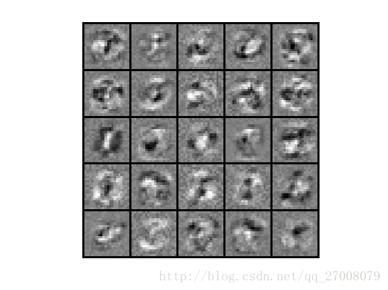
%% ================= Part 9: Visualize Weights =================
%  You can now "visualize" what the neural network is learning by 
%  displaying the hidden units to see what features they are capturing in 
%  the data.

fprintf('\nVisualizing Neural Network... \n')

displayData(Theta1(:, 2:end));

fprintf('\nProgram paused. Press enter to continue.\n');
pause;

%% ================= Part 10: Implement Predict =================
%  After training the neural network, we would like to use it to predict
%  the labels. You will now implement the "predict" function to use the
%  neural network to predict the labels of the training set. This lets
%  you compute the training set accuracy.

pred = predict(Theta1, Theta2, X);

fprintf('\nTraining Set Accuracy: %f\n', mean(double(pred == y)) * 100);

nnCostFunction.m

function [J grad] = nnCostFunction(nn_params, ...
                                   input_layer_size, ...
                                   hidden_layer_size, ...
                                   num_labels, ...
                                   X, y, lambda)
%NNCOSTFUNCTION Implements the neural network cost function for a two layer
%neural network which performs classification
%   [J grad] = NNCOSTFUNCTON(nn_params, hidden_layer_size, num_labels, ...
%   X, y, lambda) computes the cost and gradient of the neural network. The
%   parameters for the neural network are "unrolled" into the vector
%   nn_params and need to be converted back into the weight matrices. 
% 
%   The returned parameter grad should be a "unrolled" vector of the
%   partial derivatives of the neural network.
%

% Reshape nn_params back into the parameters Theta1 and Theta2, the weight matrices
% for our 2 layer neural network
Theta1 = reshape(nn_params(1:hidden_layer_size * (input_layer_size + 1)), ...
                 hidden_layer_size, (input_layer_size + 1));

Theta2 = reshape(nn_params((1 + (hidden_layer_size * (input_layer_size + 1))):end), ...
                 num_labels, (hidden_layer_size + 1));

% Setup some useful variables
m = size(X, 1);

% You need to return the following variables correctly 
J = 0;
Theta1_grad = zeros(size(Theta1));
Theta2_grad = zeros(size(Theta2));

% ====================== YOUR CODE HERE ======================
% Instructions: You should complete the code by working through the
%               following parts.
%
% Part 1: Feedforward the neural network and return the cost in the
%         variable J. After implementing Part 1, you can verify that your
%         cost function computation is correct by verifying the cost
%         computed in ex4.m
%
% Part 2: Implement the backpropagation algorithm to compute the gradients
%         Theta1_grad and Theta2_grad. You should return the partial derivatives of
%         the cost function with respect to Theta1 and Theta2 in Theta1_grad and
%         Theta2_grad, respectively. After implementing Part 2, you can check
%         that your implementation is correct by running checkNNGradients
%
%         Note: The vector y passed into the function is a vector of labels
%               containing values from 1..K. You need to map this vector into a 
%               binary vector of 1's and 0's to be used with the neural network
%               cost function.
%
%         Hint: We recommend implementing backpropagation using a for-loop
%               over the training examples if you are implementing it for the 
%               first time.
%
% Part 3: Implement regularization with the cost function and gradients.
%
%         Hint: You can implement this around the code for
%               backpropagation. That is, you can compute the gradients for
%               the regularization separately and then add them to Theta1_grad
%               and Theta2_grad from Part 2.
%
X = [ones(m, 1) X];
ylabel = zeros(num_labels, m);
for i=1:m
    ylabel(y(i), i) = 1;
end

z2 = X*Theta1';
z2 = [ones(m, 1) z2];
a2 = sigmoid(X*Theta1');
a2 = [ones(m, 1) a2];
a3 = sigmoid(a2*Theta2');

for i=1:m
    J = J - log(a3(i, :))*ylabel(:, i) - (log(1 - a3(i, :)) * (1 - ylabel(:, i)));
end
J = J/m;

J = J + lambda/2/m * (sum(sum(Theta1(:, 2:end).^2)) + sum(sum(Theta2(:, 2:end).^2)));

Delta1 = zeros(size(Theta1));
Delta2 = zeros(size(Theta2));
for t = 1:m
    delta3 = a3(t, :)' - ylabel(:, t);
    delta2 = Theta2'*delta3 .* sigmoidGradient(z2(t, :)');

    Delta1 = Delta1 + delta2(2:end) * X(t, :);
    Delta2 = Delta2 + delta3 * a2(t, :);
end

Theta1_grad = Delta1 / m;
Theta1_grad(:, 2:end) = Theta1_grad(:, 2:end) + lambda/m*Theta1(:, 2:end);
Theta2_grad = Delta2 / m;
Theta2_grad(:, 2:end) = Theta2_grad(:, 2:end) + lambda/m*Theta2(:, 2:end);
% -------------------------------------------------------------

% =========================================================================

% Unroll gradients

grad = [Theta1_grad(:) ; Theta2_grad(:)];

end

sigmoidGradient.m

function g = sigmoidGradient(z)
%SIGMOIDGRADIENT returns the gradient of the sigmoid function
%evaluated at z
%   g = SIGMOIDGRADIENT(z) computes the gradient of the sigmoid function
%   evaluated at z. This should work regardless if z is a matrix or a
%   vector. In particular, if z is a vector or matrix, you should return
%   the gradient for each element.

g = zeros(size(z));

% ====================== YOUR CODE HERE ======================
% Instructions: Compute the gradient of the sigmoid function evaluated at
%               each value of z (z can be a matrix, vector or scalar).


g = sigmoid(z).*(1 - sigmoid(z));
% =============================================================

end

randInitializeWeights.m

function W = randInitializeWeights(L_in, L_out)
%RANDINITIALIZEWEIGHTS Randomly initialize the weights of a layer with L_in
%incoming connections and L_out outgoing connections
%   W = RANDINITIALIZEWEIGHTS(L_in, L_out) randomly initializes the weights 
%   of a layer with L_in incoming connections and L_out outgoing 
%   connections. 
%
%   Note that W should be set to a matrix of size(L_out, 1 + L_in) as
%   the first column of W handles the "bias" terms
%

% You need to return the following variables correctly 
W = zeros(L_out, 1 + L_in);

% ====================== YOUR CODE HERE ======================
% Instructions: Initialize W randomly so that we break the symmetry while
%               training the neural network.
%
% Note: The first column of W corresponds to the parameters for the bias unit
%

epsilon = 0.12;
W = rand(L_out, 1+L_in)*2*epsilon - epsilon;


% =========================================================================

end

这里写图片描述

Coursera吴恩达机器学习课程总结笔记及作业代码——第5周神经网络续

Neural Networks:Learning

1.1 Cost function

1.2 Backpropagation algorithm

1.3 Unrolling parameters

1.4 Gradient checking

1.5 Random initalization

2. 程序代码

猜你喜欢

Coursera吴恩达机器学习课程 总结笔记及作业代码——第5周神经网络续

Neural Networks:Learning

1.1 Cost function

1.2 Backpropagation algorithm

1.3 Unrolling parameters

1.4 Gradient checking

1.5 Random initalization

2. 程序代码

猜你喜欢

Coursera吴恩达机器学习课程总结笔记及作业代码——第5周神经网络续