对于单特征问题上篇采用梯度下降优化θ,其实单特征和多特征甚至包括后面的逻辑回归梯度下降优化算法思想几乎是完全一样的,区别的仅是假设函数。
虽然都不提倡自己写优化算法,但在练习的时候自己写一下还是很有必要的,对理论理解的偏差在代码中会无限放大放大。。。
正规方程的优势:在于不需要找学习率、不需要设定阀值、不需要多次迭代,集万千宠爱于一身,简单快捷一次出结果
正规方程缺点:只能在线性回归中使用
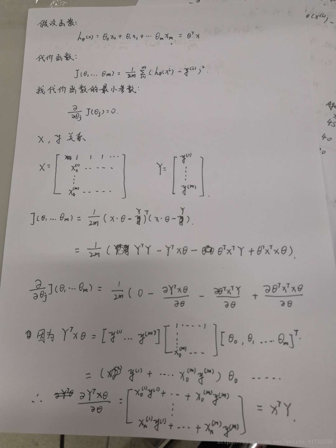
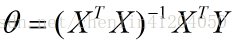
正规方程:
这个是直接可以用的。 顺便把手推在最后发一下。
手撕代码系列:
简单将Andrew Ng教授视频的例子代码实现。还是采用两种方式,一个是手写优化算法,一种采用sklearn库
# -*-coding:utf-8-*-
import numpy as np

x = np.mat([[1, 2.1, 5, 1, 45], [1, 1.4, 3, 2, 40], [1, 1.5, 3, 2, 30], [1, 8.5, 2, 1, 36], [1, 7.3, 2, 1, 40]])
print x
y = np.mat([4.6, 2.3, 3.1, 4.7, 1.5])
print y.T
# 求xTx
ts_x = np.dot(x.T, x)
print  ts_x
if np.linalg.det(ts_x) != 0:
    counter_ts_x = np.linalg.inv(ts_x)
else:
    counter_ts_x = np.linalg.pinv(ts_x)
print counter_ts_x
# (xT*x)-1*x
ctx_x = counter_ts_x * x.T
print ctx_x
calculate_y = ctx_x * y.T
print calculate_y
# [[-35.29425287]
#  [  2.48275862]
#  [  5.42873563]
#  [ 10.01954023]
#  [ -0.05517241]]
sklearn
x = [(1, 2.1, 5, 1, 45), (1, 1.4, 3, 2, 40), (1, 1.5, 3, 2, 30), (1, 8.5, 2, 1, 36), (1, 7.3, 2, 1, 40)]
# y[i] 样本点对应的输出
y = [4.6, 2.3, 3.1, 4.7, 1.5]

from sklearn.linear_model import LinearRegression
lr = LinearRegression()
lr.fit(x,y)
print lr.coef_,lr.intercept_
# [ 0.          2.48275862  5.42873563 10.01954023 -0.05517241] -35.29425287356317
以上两个θ完全相同
附手推正规方程和多元梯度下降
感谢李永乐老师的线代课,哈哈哈