实例1:

#!/usr/bin/env python3
# -*- coding: utf-8 -*-

import tensorflow as tf
import numpy as np

# 模拟生成100对数据对, 对应的函数为y = x * 0.1 + 0.3
x_data = np.random.rand(100).astype("float32")
y_data = x_data * 0.1 + 0.3

# 指定w和b变量的取值范围（利用TensorFlow来得到w和b的值）
W = tf.Variable(tf.random_uniform([1], -1.0, 1.0)) #随机生成一个在[-1,1]范围的均匀分布数值
b = tf.Variable(tf.zeros([1])) #set b=0
y = W * x_data + b

# 最小化均方误差
loss = tf.reduce_mean(tf.square(y - y_data))
optimizer = tf.train.GradientDescentOptimizer(0.5) #学习率为0.5的梯度下降法
train = optimizer.minimize(loss)

# 初始化TensorFlow参数
init = tf.initialize_all_variables()

# 运行数据流图（
sess = tf.Session()
sess.run(init)

# 观察多次迭代计算时，w和b的拟合值
for step in range(201):
    sess.run(train)
    if step % 20 == 0:
        print(step, sess.run(W), sess.run(b))

注释：上面代码是要拟合出直线: y=0.1x+0.3，算法原理很简单，就是先初始化一个w和b，然后逐步迭代（代码中用的是学习率为0.5的梯度下降法），使得y和y_data的均方误差最小，主要是学习TensorFlow的实现方法。这里附tf.reduce_mean( )的函数说明：

函数作用：
沿着tensor的某一维度，计算元素的平均值。由于输出tensor的维度比原tensor的低，这类操作也叫降维。
参数：
reduce_mean(input_tensor,axis=None,keep_dims=False,name=None, reduction_indices=None)
input_tensor：需要降维的tensor。
axis：axis=none, 求全部元素的平均值；axis=0, 按列降维，求每列平均值；axis=1，按行降维，求每行平均值。
keep_dims：若值为True，可多行输出平均值。
name：自定义操作的名称。
reduction_indices：axis的旧名，已停用。

上面代码执行结果：

0 [ 0.60980111] [ 0.0624467]
20 [ 0.25957468] [ 0.22225133]
40 [ 0.15037055] [ 0.27545825]
60 [ 0.11589972] [ 0.29225329]
80 [ 0.10501883] [ 0.2975547]
100 [ 0.10158423] [ 0.29922813]
120 [ 0.10050007] [ 0.29975638]
140 [ 0.10015786] [ 0.29992309]
160 [ 0.10004983] [ 0.29997572]
180 [ 0.10001571] [ 0.29999235]
200 [ 0.10000496] [ 0.2999976]

迭代到200步时，w和b的值已经接近于最佳。

拟合实质上和回归是一样的，为了更加直观的显示迭代过程中每次拟合的情况，使用matplotlib把图绘制出来，见实例2。

实例2：

#!/usr/bin/env python3
# -*- coding: utf-8 -*-

import numpy as np
import matplotlib.pyplot as plt

num_points = 1000
vectors_set = []
for i in range(num_points):
     x1= np.random.normal(0.0, 0.55)
     y1= x1 * 0.1 + 0.3 + np.random.normal(0.0, 0.03)
     vectors_set.append([x1, y1])

x_data = [v[0] for v in vectors_set]
y_data = [v[1] for v in vectors_set]



#Graphic display
plt.plot(x_data, y_data, 'ro')
plt.legend()
plt.show()

import tensorflow as tf

W = tf.Variable(tf.random_uniform([1], -1.0, 1.0))
b = tf.Variable(tf.zeros([1]))
y = W * x_data + b

loss = tf.reduce_mean(tf.square(y - y_data))
optimizer = tf.train.GradientDescentOptimizer(0.5)
train = optimizer.minimize(loss)

init = tf.initialize_all_variables()

sess = tf.Session()
sess.run(init)

for step in range(101):
     sess.run(train)
     if step % 20 == 0:
         print(step, sess.run(W), sess.run(b))
         print(step, sess.run(loss))

         #Graphic display
         plt.plot(x_data, y_data, 'ro')
         plt.plot(x_data, sess.run(W) * x_data + sess.run(b))
         plt.xlabel('x')
         plt.xlim(-2,2)
         plt.ylim(0.1,0.6)
         plt.ylabel('y')
         plt.legend()
         plt.show()

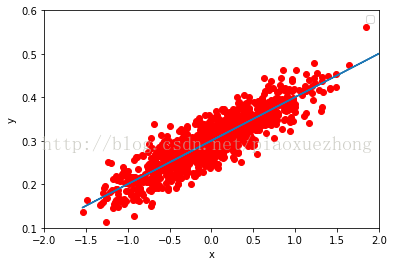
执行结果（这里只附1,2,7步的图，中间几步的图结果越来越靠近第7步）：

最后的拟合参数为：

100 [ 0.09993903] [ 0.30052763]
100 0.00088246

附录:

生成数据时的分布情况，如正态分布，均匀分布等

Operation	Description
tf.random_normal	Random values with a normal distribution
tf.truncated_normal	Random values with a normal distribution but eliminating those values whose magnitude is more than 2 times the standard deviation
tf.random_uniform	Random values with a uniform distribution
tf.random_shuffle	Randomly mixed tensor elements in the first dimension
tf.set_random_seed	Sets the random seed

实例3：

import tensorflow as tf
import numpy as np
import matplotlib.pyplot as plt

# Prepare training data
datasize=100
train_X = np.linspace(0,np.pi, datasize)
train_Y=np.sin(train_X)
# Define the model
X1 = tf.placeholder(tf.float32,shape=(datasize,))
X2 = tf.placeholder(tf.float32,shape=(datasize,))
X3 = tf.placeholder(tf.float32,shape=(datasize,))
X4 = tf.placeholder(tf.float32,shape=(datasize,))
Y = tf.placeholder(tf.float32,shape=(datasize,))
w1 = tf.Variable(0.0,name="weight1")
w2 = tf.Variable(0.0, name="weight2")
w3 = tf.Variable(0.0, name="weight3")
w4 = tf.Variable(0.0, name="weight4")

y1=w1*X1+w2*X2+w3*X3+w4*X4
loss = tf.reduce_mean(tf.square(Y - y1))
#use adam method to optimize
optimizer =tf.train.AdamOptimizer()
train=optimizer.minimize(loss)

# Create session to run
with tf.Session() as sess:
    init=tf.global_variables_initializer()
    sess.run(init)
    for i in range(5000):
        _,ww1, ww2,ww3,ww4,loss_= sess.run([train, w1, w2,w3,w4,loss],feed_dict={X1:train_X,X2:train_X**3,X3:train_X**5,X4:train_X**7,Y: train_Y})

plt.plot(train_X,train_Y,"+",label='data')
plt.plot(train_X,ww1*train_X+(ww2)*(train_X**3)+ww3*(train_X**5)+ww4*(train_X**7),label='curve')
plt.savefig('1.png',dpi=200)
plt.axis([0,np.pi,-2,2])
plt.legend(loc=1)
plt.show()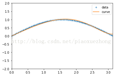

实例4：

定义张量和损失函数时，除了上面的方法，还可以写成下面的形式，本质是一样的：

import tensorflow as tf
import numpy as np
import matplotlib.pyplot as plt
# 设置带噪声的线性数据
num_examples = 50
# 这里会生成一个完全线性的数据
X = np.array([np.linspace(-2, 4, num_examples), np.linspace(-6, 6, num_examples)])
# 数据展示
plt.figure(figsize=(4,4))
plt.scatter(X[0], X[1])
plt.show

# 给数据增加噪声
X += np.random.randn(2, num_examples)
# 数据展示
plt.figure(figsize=(4,4))
plt.scatter(X[0], X[1])
plt.show

# 我们的目标就是通过学习，找到一条拟合曲线，去还原最初的线性数据
# 把数据分离成 x 和 y
x, y = X
# 添加固定为 1 的 bias
x_with_bias = np.array([(1., a) for a in x]).astype(np.float32)
# 用来记录每次迭代的 loss
losses = []
# 迭代次数
training_steps = 50
# 学习率，梯度下降时每次迭代所前进的长度
learning_rate = 0.002

with tf.Session() as sess:
    # 设置所有的张量，变量和操作
    # 输入层是 x 值和 bias 节点
    input = tf.constant(x_with_bias)
    # target 是 y 的值，需要被调整成正确的尺寸（转置一下）
    target = tf.constant(np.transpose([y]).astype(np.float32))
    # weights 是变量，每次循环都会变，这里直接随机初始化（高斯分布，均值 0，标准差 0.1）
    weights = tf.Variable(tf.random_normal([2, 1], 0, 0.1))

    # 初始化所有的变量
    tf.global_variables_initializer().run()

    # 设置循环中所要做的全部操作
    # 对于所有的 x，根据现有的 weights 来产生对应的 y 值，也就是计算 y = w2 * x + w1 * bias
    yhat = tf.matmul(input, weights)
    yerror = tf.subtract(yhat, target)
    # 最小化 L2 损失，误差的平方
    loss = tf.nn.l2_loss(yerror)
    # 上面的 loss 函数相当于0.5 * tf.reduce_sum(tf.multiply(yerror, yerror))

    update_weights = tf.train.GradientDescentOptimizer(learning_rate).minimize(loss)
    # 上面的梯度下降相当于
    # gradient = tf.reduce_sum(tf.transpose(tf.multiply(input, yerror)), 1, keep_dims=True)
    # update_weights = tf.assign_sub(weights, learning_rate * gradient)

    for _ in range(training_steps):
        update_weights.run()
        # 如果没有用 tf.train.GradientDescentOptimizer，就要 sess.run(update_weights)
        losses.append(loss.eval())

    # 训练结束
    betas = weights.eval()
    yhat = yhat.eval()
    

fig, (ax1, ax2) = plt.subplots(1, 2)
plt.subplots_adjust(wspace=.3)
fig.set_size_inches(10, 4)
ax1.scatter(x, y, alpha=.7)
ax1.scatter(x, np.transpose(yhat)[0], c="g", alpha=.6)
line_x_range = (-4, 6)
ax1.plot(line_x_range, [betas[0] + a * betas[1] for a in line_x_range], "g", alpha=.6)
ax2.plot(range(0, training_steps), losses)
ax2.set_ylabel("Loss")
ax2.set_xlabel("Training steps")
plt.show()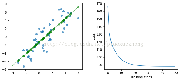

运行结果：

参考：

https://www.tensorflow.org/get_started/get_started

http://www.jeyzhang.com/tensorflow-learning-notes.html

http://wdxtub.com/2017/05/31/tensorflow-learning-note/

http://jorditorres.org/research-teaching/tensorflow/first-contact-with-tensorflow-book/first-contact-with-tensorflow/#cap1

tensorflow学习笔记（3）梯度下降法进行曲线拟合和线性回归

实例1:

实例2：

实例3：

实例4：

猜你喜欢