数字图像处理笔记（八）：频域高通滤波锐化图像

1 - 引言

在笔记（七）中，我们通过衰减图像的傅里叶变换的高频成分来平滑对象，因为边缘和其他灰度的急剧变化与高频分量有关，所以图像的锐化可在频域通过高通滤波来实现。
一个高通滤波器是从给定的低通滤波器用下式得到：
$H_{HP}(u,v)=1-H_{LP}(u,v)$
其中， $H_{LP}(u，v)$是低通滤波器的传递函数，也就是说之前介绍的三种低通滤波器：理想、布特沃斯、高斯低通滤波器可以通过上面的式子快速的转变为高通滤波器。接下来，我们介绍其他的高通滤波器

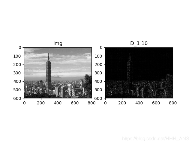
2 - 频率域的拉普拉斯算子

拉普拉斯算子可使用如下滤波器在频率域中实现：
$H(u,v)=-4\pi^2(u^2+v^2)$
在关于频率矩形的中心，使用如下滤波器：
$H(u,v)=-4\pi^2[(u-p/2)^2+(v-Q/s)^2]=-4\pi^2D^2(u,v)$
其中，D(u,v)是距离函数。

import cv2
import numpy as np
import matplotlib.pyplot as plt

img = cv2.imread('images/12.jpg',0) #直接读为灰度图像
f = np.fft.fft2(img)
fshift = np.fft.fftshift(f)
s1 = np.log(np.abs(fshift))


def LaplaceFilter(image,d):
    f = np.fft.fft2(image)
    fshift = np.fft.fftshift(f)
    def make_transform_matrix(d):
        transfor_matrix = np.zeros(image.shape)
        center_point = tuple(map(lambda x:(x-1)/2,s1.shape))
        for i in range(transfor_matrix.shape[0]):
            for j in range(transfor_matrix.shape[1]):
                def cal_distance(pa,pb):
                    from math import sqrt
                    dis = sqrt((pa[0]-pb[0])**2+(pa[1]-pb[1])**2)
                    return dis
                dis = cal_distance(center_point,(i,j))
                transfor_matrix[i,j] = -4*(np.pi**2)*(dis**2)
        return transfor_matrix
    d_matrix = make_transform_matrix(d)
    new_img = np.abs(np.fft.ifft2(np.fft.ifftshift(fshift*d_matrix)))
    return new_img

img_d1 = LaplaceFilter(img,10)
plt.title('D_1 10')
plt.imshow(img_d1,cmap="gray")
plt.show()

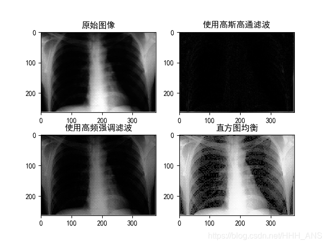
3 - 高频强调滤波

使用频率域方法，模板由下式：
$g_mask(x,y)=f(x,y)-f_{LP}(x,y)$
和
$f_{LP}(x,y)=\Im^{-1}[H_{LP}(u,v)F(u,v)]$
其中， $H_{LP}(u,v)$是一个低通滤波器， $F(u,v)$是f(x,y)的傅里叶变换。 $f_{LP}(x,y)$是平滑后的图像，类似于f(x,y)。然后又 $g(x,y)=f(x,y)+k*g_{mask}(x,y)$
该表达式定义了k=1时的钝化模板和k>1时的高提升滤波器。
$g(x,y)=\Im^{-1}\left \{ [1+k*[1-H_{LP}(u,v)]]F(u,v) \right \}$
由 $H_{HP}(u,v)=1-H_{LP}(u,v)$得
$g(x,y)=\Im^{-1}\left \{ [1+k*H_{HP}(u,v)]]F(u,v) \right \}$
方括号中的表达式，即 $1+k*H_{HP}(u,v)$成为高频强调滤波器。
高频强调滤波器更一般的公式为
$g(x,y)=\Im^{-1}\left \{ [k_1+k_2*H_{HP}(u,v)]]F(u,v) \right \}$

其中， $k_1\geq 0$ 给出了控制距原点的偏移量， $k_2\geq$控制高频的贡献。

import cv2
import numpy as np
import matplotlib.pyplot as plt

#解决中文显示问题
plt.rcParams['font.sans-serif']=['SimHei']
plt.rcParams['axes.unicode_minus'] = False

img = cv2.imread('images/test_5.jpg',0) #直接读为灰度图像
f = np.fft.fft2(img)
fshift = np.fft.fftshift(f)
s1 = np.log(np.abs(fshift))

def GaussianLowFilter(image,d,flag=None):
    f = np.fft.fft2(image)
    fshift = np.fft.fftshift(f)
    def make_transform_matrix(d):
        transfor_matrix = np.zeros(image.shape)
        center_point = tuple(map(lambda x:(x-1)/2,s1.shape))
        for i in range(transfor_matrix.shape[0]):
            for j in range(transfor_matrix.shape[1]):
                def cal_distance(pa,pb):
                    from math import sqrt
                    dis = sqrt((pa[0]-pb[0])**2+(pa[1]-pb[1])**2)
                    return dis
                dis = cal_distance(center_point,(i,j))
                if flag == 0:
                    transfor_matrix[i,j] =0.5+0.75*(1-np.exp(-(dis**2)/(2*(d**2))))
                else:
                    transfor_matrix[i, j] = 1 - np.exp(-(dis ** 2) / (2 * (d ** 2)))
        return transfor_matrix
    d_matrix = make_transform_matrix(d)
    new_img = np.abs(np.fft.ifft2(np.fft.ifftshift(fshift*d_matrix)))
    return new_img

plt.subplot(221)
plt.imshow(img,cmap="gray")
plt.title("原始图像")

plt.subplot(222)
img_d1 = GaussianLowFilter(img,40,1)
plt.imshow(img_d1,cmap="gray")
plt.title('使用高斯高通滤波')

plt.subplot(223)
img_d2 = GaussianLowFilter(img,40,0)
plt.imshow(img_d2,cmap="gray")
plt.title('使用高频强调滤波')
"""
因为进过傅里叶变换图像的像素变成了浮点型，但是直方图均衡
函数的输入数据为整形，所以需要进行数据类型转换
"""
plt.subplot(224)
img_d3 = GaussianLowFilter(img,40,0)
img_d3 = img_d3.astype(np.uint8)
img_d3=cv2.equalizeHist(img_d3)
plt.imshow(img_d3,cmap="gray")
plt.title('直方图均衡')
plt.show()

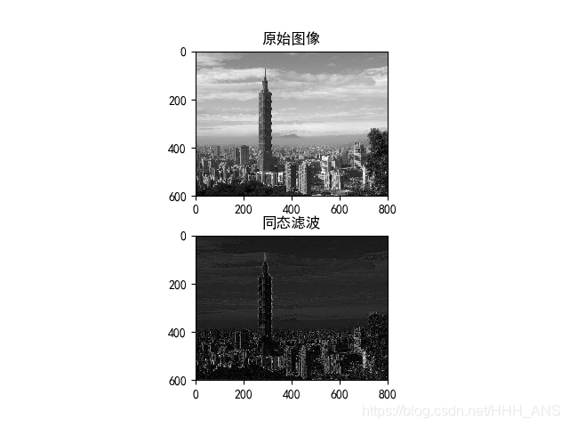
4 - 同态滤波

在生活中会得到这样的图像，动态范围很大，感兴趣的部分的灰度却很暗，范围很小，灰度层次和细节没有办法辨认，用一般的灰度线性变换法是不行的，因为扩展灰度级虽可以提高物体图像的 因为扩展灰度级虽可以提高物体图像的反差，但会使动态范围变大。而压缩灰 反差，但会使动态范围变大。而压缩灰度级，虽可以减少动态范围，但物体灰 度级，虽可以减少动态范围，但物体灰
度层次和细节就会更看不清。 度层次和细节就会更看不．这时我们需要采用同态滤波。同态滤波是一种在频域中同时将图像亮度范围进行压缩和将图像对比度进行增强的方法。

同态滤波

节选自百度百科里的一段话：同态滤波的基本原理是：将像元灰度值看作是照度和反射率两个组份的产物。由于照度相对变化很小，可以看作是图像的低频成份，而反射率则是高频成份。通过分别处理照度和反射率对像元灰度值的影响，达到揭示阴影区细节特征的目的。同态滤波处理的基本流程如下：

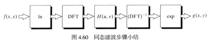
其中f(x,y)为原始图像，ln为对数变换，DFT为傅里叶变换，H（u,v）为频域滤波， $(DFT)^{-1}$为傅里叶逆变换，exp为指数运算，g(x,y)为输出图像。

图片的照射分量通常由慢的空间变化来表征，而反射分量往往引起突变，特变是在不同物体的连接部分。这些特性导致图像取对数后的傅里叶变换的低频成分与照射相联系，而高频成分与反射相联系。虽然这些联系知识粗略的近似，但它们用在图像滤波中是有益的。

使用同态滤波器可更好地控制照射分量和反射分量，这种控制需要指定一个滤波器函数H（u,v）,它可用不同的可控方法影响傅里叶变换的低频和高频分量。

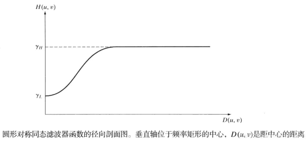
这个函数形状可以用高通滤波器的基本形式来近似。
$H(u,v)=(\gamma_H-\gamma_L)[1-\exp^{c[D^2(u,v)/D^2_0]}]+\gamma_L$

import cv2
import numpy as np
import matplotlib.pyplot as plt

#解决中文显示问题
plt.rcParams['font.sans-serif']=['SimHei']
plt.rcParams['axes.unicode_minus'] = False

img = cv2.imread('images/12.jpg',0) #直接读为灰度图像
f = np.fft.fft2(img)
fshift = np.fft.fftshift(f)
s1 = np.log(np.abs(fshift))


def Homomorphic(image,d,L,H,c):
    f = np.fft.fft2(image)
    fshift = np.fft.fftshift(f)
    def make_transform_matrix(d,L,H,c):
        transfor_matrix = np.zeros(image.shape)
        center_point = tuple(map(lambda x:(x-1)/2,s1.shape))
        for i in range(transfor_matrix.shape[0]):
            for j in range(transfor_matrix.shape[1]):
                def cal_distance(pa,pb):
                    from math import sqrt
                    dis = sqrt((pa[0]-pb[0])**2+(pa[1]-pb[1])**2)
                    return dis
                dis = cal_distance(center_point,(i,j))
                transfor_matrix[i,j] = (H-L)*(1-np.exp(-c*(dis**2/d**2)))+L
        return transfor_matrix
    d_matrix = make_transform_matrix(d,L,H,c)
    new_img = np.abs(np.fft.ifft2(np.fft.ifftshift(fshift*d_matrix)))
    return new_img

plt.subplot(211)
plt.title('原始图像')
plt.imshow(img,cmap="gray")

plt.subplot(212)
img_d1 = Homomorphic(img,80,0.25,2,1)
plt.title('同态滤波')
plt.imshow(img_d1,cmap="gray")
plt.show()

5 - 小结

本文主要介绍了各种频域的高通滤波器来对图像进行处理，可以看到高通滤波器主要是将图片中的边缘提取出来，让图片的细节更加清晰。高通和低通滤波器的相互转换也十分方便，通过灵活的集合各种滤波器可以帮助我们清除图像的噪音并且把我们感兴趣的细节提取出来。