版权声明:本文为博主原创文章,未经博主允许不得转载。 https://blog.csdn.net/u013817676/article/details/79004863
使用keras的深度学习来分类白葡萄酒还是红葡萄酒
首先介绍一下数据类型:
1.这个数据集包含了1599种红酒,4898种白酒;
2.输入数据特征:
1 - fixed acidity
2 - volatile acidity
3 - citric acid
4 - residual sugar
5 - chlorides
6 - free sulfur dioxide
7 - total sulfur dioxide
8 - density
9 - pH
10 - sulphates
11 - alcohol
3.输出变量:
12 - quality (score between 0 and 10)
import pandas as pd
#导入数据
white = pd.read_csv("http://archive.ics.uci.edu/ml/machine-learning-databases/wine-quality/winequality-white.csv", sep=';')

red = pd.read_csv("http://archive.ics.uci.edu/ml/machine-learning-databases/wine-quality/winequality-red.csv", sep=';')
#查看白酒信息
print white.info()<class 'pandas.core.frame.DataFrame'>
RangeIndex: 4898 entries, 0 to 4897
Data columns (total 12 columns):
fixed acidity 4898 non-null float64
volatile acidity 4898 non-null float64
citric acid 4898 non-null float64
residual sugar 4898 non-null float64
chlorides 4898 non-null float64
free sulfur dioxide 4898 non-null float64
total sulfur dioxide 4898 non-null float64
density 4898 non-null float64
pH 4898 non-null float64
sulphates 4898 non-null float64
alcohol 4898 non-null float64
quality 4898 non-null int64
dtypes: float64(11), int64(1)
memory usage: 459.3 KB
None
#查看红酒信息
print red.info()
<class 'pandas.core.frame.DataFrame'>
RangeIndex: 1599 entries, 0 to 1598
Data columns (total 12 columns):
fixed acidity 1599 non-null float64
volatile acidity 1599 non-null float64
citric acid 1599 non-null float64
residual sugar 1599 non-null float64
chlorides 1599 non-null float64
free sulfur dioxide 1599 non-null float64
total sulfur dioxide 1599 non-null float64
density 1599 non-null float64
pH 1599 non-null float64
sulphates 1599 non-null float64
alcohol 1599 non-null float64
quality 1599 non-null int64
dtypes: float64(11), int64(1)
memory usage: 150.0 KB
None
#查看具体值
print red.head()
fixed acidity volatile acidity citric acid residual sugar chlorides \
0 7.4 0.70 0.00 1.9 0.076
1 7.8 0.88 0.00 2.6 0.098
2 7.8 0.76 0.04 2.3 0.092
3 11.2 0.28 0.56 1.9 0.075
4 7.4 0.70 0.00 1.9 0.076
free sulfur dioxide total sulfur dioxide density pH sulphates \
0 11.0 34.0 0.9978 3.51 0.56
1 25.0 67.0 0.9968 3.20 0.68
2 15.0 54.0 0.9970 3.26 0.65
3 17.0 60.0 0.9980 3.16 0.58
4 11.0 34.0 0.9978 3.51 0.56
alcohol quality
0 9.4 5
1 9.8 5
2 9.8 5
3 9.8 6
4 9.4 5
#查看各行统计信息
print red.describe()
fixed acidity volatile acidity citric acid residual sugar \
count 1599.000000 1599.000000 1599.000000 1599.000000
mean 8.319637 0.527821 0.270976 2.538806
std 1.741096 0.179060 0.194801 1.409928
min 4.600000 0.120000 0.000000 0.900000
25% 7.100000 0.390000 0.090000 1.900000
50% 7.900000 0.520000 0.260000 2.200000
75% 9.200000 0.640000 0.420000 2.600000
max 15.900000 1.580000 1.000000 15.500000
chlorides free sulfur dioxide total sulfur dioxide density \
count 1599.000000 1599.000000 1599.000000 1599.000000
mean 0.087467 15.874922 46.467792 0.996747
std 0.047065 10.460157 32.895324 0.001887
min 0.012000 1.000000 6.000000 0.990070
25% 0.070000 7.000000 22.000000 0.995600
50% 0.079000 14.000000 38.000000 0.996750
75% 0.090000 21.000000 62.000000 0.997835
max 0.611000 72.000000 289.000000 1.003690
pH sulphates alcohol quality
count 1599.000000 1599.000000 1599.000000 1599.000000
mean 3.311113 0.658149 10.422983 5.636023
std 0.154386 0.169507 1.065668 0.807569
min 2.740000 0.330000 8.400000 3.000000
25% 3.210000 0.550000 9.500000 5.000000
50% 3.310000 0.620000 10.200000 6.000000
75% 3.400000 0.730000 11.100000 6.000000
max 4.010000 2.000000 14.900000 8.000000
import numpy as np
#查看是否有数据缺失
print np.any(red.isnull()==True)
False
print np.any(white.isnull()==True)False
#可视化数据
import matplotlib.pyplot as plt

fig,ax = plt.subplots(1,2)

ax[0].hist(red.alcohol, 10, facecolor='red', alpha=0.5, label="Red wine")
ax[1].hist(white.alcohol, 10, facecolor='white', ec="black", lw=0.5, alpha=0.5, label="White wine")

fig.subplots_adjust(left=0, right=1, bottom=0, top=0.5, hspace=0.05, wspace=1)
ax[0].set_ylim([0, 1000])
ax[0].set_xlabel("Alcohol in % Vol")
ax[0].set_ylabel("Frequency")
ax[1].set_xlabel("Alcohol in % Vol")
ax[1].set_ylabel("Frequency")
ax[0].legend(loc='best')
ax[1].legend(loc='best')
fig.suptitle("Distribution of Alcohol in % Vol")

plt.show()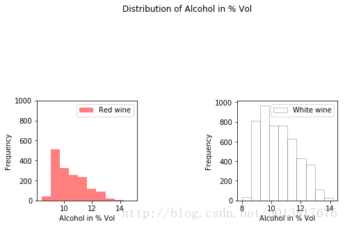
我们可以从图中看出红酒和白酒的酒精浓度基本上9%左右。
#处理数据
#给我们的数据添加标签
red['label'] = 1
white['label'] = 0
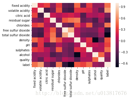
wines = red.append(white,ignore_index=True) #合并index顺序import seaborn as sns
%matplotlib inline
corr = wines.corr() #计算协方差
sns.heatmap(corr,
xticklabels = corr.columns.values,
yticklabels = corr.columns.values)
sns.plt.show() #plt.show()---------------------------------------------------------------------------
AttributeError Traceback (most recent call last)
<ipython-input-18-5a30364cdd9b> in <module>()
5 xticklabels = corr.columns.values,
6 yticklabels = corr.columns.values)
----> 7 sns.plt.show()
AttributeError: 'module' object has no attribute 'plt'
这边改成plt.show()就不会报错了!
从图中我们可以看到各个特征之间的相关性,从中我们可以发现density跟residual sugar是正相关的,而跟alcohol是负相关的。
#划分训练集合测试集
from sklearn.model_selection import train_test_split
X = wines.iloc[:,0:11]
y = np.ravel(wines.label) #降成一维,类似np.flatten(),但是np.flatten是拷贝,而ravel是引用

#随机划分训练集和测试集
#test_size:测试集占比
#random_state:随机种子,在需要重复试验的时候,保证得到一组一样的随机数。
X_train,X_test,y_train,y_test = train_test_split(X,y,test_size=0.33, random_state=32)
#标准化数据
from sklearn.preprocessing import StandardScaler
scaler = StandardScaler().fit(X_train)
X_train = scaler.transform(X_train)
X_test = scaler.transform(X_test)#使用keras模型化数据
from keras.models import Sequential
from keras.layers import Dense
model = Sequential()
#添加输入层
model.add(Dense(12,activation='relu',
input_shape=(11,)))
#添加隐藏层
model.add(Dense(8,activation='relu'))
#添加输出层
model.add(Dense(1,activation='sigmoid'))Using TensorFlow backend.
#查看模型
#查看输出维度
print model.output_shape
(None, 1)
#查看整个模型
print model.summary()
_________________________________________________________________
Layer (type) Output Shape Param #
=================================================================
dense_1 (Dense) (None, 12) 144
_________________________________________________________________
dense_2 (Dense) (None, 8) 104
_________________________________________________________________
dense_3 (Dense) (None, 1) 9
=================================================================
Total params: 257
Trainable params: 257
Non-trainable params: 0
_________________________________________________________________
None
#查看模型参数
print model.get_weights()
#模型的训练
model.compile(loss='binary_crossentropy',
optimizer='adam',
metrics=['accuracy'])
#verbose = 1 查看输出过程
model.fit(X_train,y_train,epochs=30,batch_size=1,verbose=1)Epoch 1/30
4352/4352 [==============================] - 15s - loss: 0.1108 - acc: 0.9614
Epoch 2/30
4352/4352 [==============================] - 15s - loss: 0.0255 - acc: 0.9952
Epoch 3/30
4352/4352 [==============================] - 15s - loss: 0.0195 - acc: 0.9954
Epoch 4/30
4352/4352 [==============================] - 15s - loss: 0.0180 - acc: 0.9966
Epoch 5/30
4352/4352 [==============================] - 15s - loss: 0.0166 - acc: 0.9966
Epoch 6/30
4352/4352 [==============================] - 15s - loss: 0.0147 - acc: 0.9970
Epoch 7/30
4352/4352 [==============================] - 15s - loss: 0.0132 - acc: 0.9968
Epoch 8/30
4352/4352 [==============================] - 15s - loss: 0.0137 - acc: 0.9970
Epoch 9/30
4352/4352 [==============================] - 16s - loss: 0.0136 - acc: 0.9975
Epoch 10/30
4352/4352 [==============================] - 15s - loss: 0.0125 - acc: 0.9975
Epoch 11/30
4352/4352 [==============================] - 15s - loss: 0.0113 - acc: 0.9972
Epoch 12/30
4352/4352 [==============================] - 15s - loss: 0.0116 - acc: 0.9972
Epoch 13/30
4352/4352 [==============================] - 15s - loss: 0.0115 - acc: 0.9975
Epoch 14/30
4352/4352 [==============================] - 15s - loss: 0.0108 - acc: 0.9972
Epoch 15/30
4352/4352 [==============================] - 16s - loss: 0.0097 - acc: 0.9975
Epoch 16/30
4352/4352 [==============================] - 16s - loss: 0.0098 - acc: 0.9977
Epoch 17/30
4352/4352 [==============================] - 15s - loss: 0.0101 - acc: 0.9975
Epoch 18/30
4352/4352 [==============================] - 15s - loss: 0.0095 - acc: 0.9970
Epoch 19/30
4352/4352 [==============================] - 15s - loss: 0.0088 - acc: 0.9977
Epoch 20/30
4352/4352 [==============================] - 16s - loss: 0.0089 - acc: 0.9972
Epoch 21/30
4352/4352 [==============================] - 16s - loss: 0.0086 - acc: 0.9977
Epoch 22/30
4352/4352 [==============================] - 16s - loss: 0.0078 - acc: 0.9982
Epoch 23/30
4352/4352 [==============================] - 16s - loss: 0.0085 - acc: 0.9979
Epoch 24/30
4352/4352 [==============================] - 15s - loss: 0.0072 - acc: 0.9984
Epoch 25/30
4352/4352 [==============================] - 16s - loss: 0.0074 - acc: 0.9982
Epoch 26/30
4352/4352 [==============================] - 15s - loss: 0.0071 - acc: 0.9986
Epoch 27/30
4352/4352 [==============================] - 16s - loss: 0.0080 - acc: 0.9977
Epoch 28/30
4352/4352 [==============================] - 16s - loss: 0.0066 - acc: 0.9982
Epoch 29/30
4352/4352 [==============================] - 16s - loss: 0.0084 - acc: 0.9982
Epoch 30/30
4352/4352 [==============================] - 15s - loss: 0.0067 - acc: 0.9989
<keras.callbacks.History at 0x120530a90>
#预测结果
y_pred = model.predict(X_test)
print y_pred[:10]
[[ 2.14960589e-03]
[ 6.35436322e-07]
[ 1.82669051e-03]
[ 2.15678483e-07]
[ 1.00000000e+00]
[ 1.84882566e-07]
[ 1.13470778e-04]
[ 5.90343404e-07]
[ 2.01183035e-08]
[ 1.00000000e+00]]
print y_test[:10][0 0 0 0 1 0 0 0 0 1]
可以从上述结果可以看出,测试集的前十项结果跟我们预测的结果是一样的。
#模型评估
score = model.evaluate(X_test,y_test,verbose=1)

#socre的两个值分别代表损失(loss)和精准度(accuracy)
print score
960/2145 [============>.................] - ETA: 0s[0.030568929157742158, 0.99580419580419577]
#统计Precision、Recall、F1值
from sklearn.metrics import confusion_matrix,precision_score,recall_score,f1_score

y_pred = y_pred.astype(int) #转化成整型
print confusion_matrix(y_test,y_pred)
[[1633 0]
[ 230 282]]
#precision
precision = precision_score(y_test,y_pred)
print precision
1.0
#Recall
recall = recall_score(y_test,y_pred)
print recall
0.55078125
#F1 score
f1 = f1_score(y_test,y_pred)
print f1
0.710327455919
从上面的结果来看我们的Precision很高,但是我们的Recall值比较低。
对此我后面还会写一篇blog来优化模型。