【王俊杰de人工智能实战课】第3次作业

Brief Guide

项目	内容
这个作业属于哪个课程	北航人工智能实战课
这个作业的要求在哪里	第三次作业要求
我在这个课程的目标是	获得机器学习相关的完整项目与学习经验；通过与人工智能行业的大牛们聊天了解行业不同方向的发展以便进行职业规划；为转CS积累基础知识并获得相关课程的成绩
这个作业在哪个具体方面帮助我实现目标	详细学习了人工智能算法中最基础、最重要的算法之一“梯度下降”的三种方法
作业正文…	【王俊杰de人工智能实战课】第3次作业
其他参考文献…	微软AI教育GitHub

Main Homework

代码解析

导入包

import numpy as np
import matplotlib.pyplot as plt
from pathlib import Path

定义数据文件名

x_data_name = "TemperatureControlXData.dat"
y_data_name = "TemperatureControlYData.dat"

定义CData类，输入损失、权重、偏移、响应、迭代次数

class CData(object):
    def __init__(self, loss, w, b, epoch, iteration):
        self.loss = loss
        self.w = w
        self.b = b
        self.epoch = epoch
        self.iteration = iteration

根据定义的文件名读取X和Y的数据，若文件不存在则返回None

def ReadData():
    Xfile = Path(x_data_name)
    Yfile = Path(y_data_name)
    if Xfile.exists() & Yfile.exists():
        X = np.load(Xfile)
        Y = np.load(Yfile)
        return X.reshape(1,-1),Y.reshape(1,-1)
    else:
        return None,None

定义前向计算公式: \(z=w*x+b\)

def ForwardCalculationBatch(W,B,batch_x):
    Z = np.dot(W, batch_x) + B
    return Z

定义反向传播公式：
\[db=\sum{\frac{z-y}{m}}\]\[dw=\frac{(z-y)*x^T}{m}\]

def BackPropagationBatch(batch_x, batch_y, batch_z):
    m = batch_x.shape[1]
    dZ = batch_z - batch_y
    dB = dZ.sum(axis=1, keepdims=True)/m
    dW = np.dot(dZ, batch_x.T)/m
    return dW, dB

更新权重，定义新的权重为：
\[w=w-\eta *dw\]\[b=b-\eta *db\]

def UpdateWeights(w, b, dW, dB, eta):
    w = w - eta*dW
    b = b - eta*dB
    return w,b

初始化权重：

若flag=0，W初始化为全0矩阵；

若flag=1，W初始化为随机标准化矩阵；

若flag=2，W初始化为随机矩阵，值为\(-\sqrt{\frac{6}{n_{in} + n_{out}}}\)或\(\sqrt{\frac{6}{n_{in} + n_{out}}}\)

B初始化为全0矩阵

def InitialWeights(num_input, num_output, flag):
    if flag == 0:
        # zero
        W = np.zeros((num_output, num_input))
    elif flag == 1:
        # normalize
        W = np.random.normal(size=(num_output, num_input))
    elif flag == 2:
        # xavier
        W=np.random.uniform(
            -np.sqrt(6/(num_input+num_output)),
            np.sqrt(6/(num_input+num_output)),
            size=(num_output,num_input))

    B = np.zeros((num_output, 1))
    return W,B

绘图，显示Y关于X的变化趋势与Z关于X的变化趋势，输出w、b和迭代次数的值

def ShowResult(X, Y, w, b, iteration):
    # draw sample data
    plt.plot(X, Y, "b.")
    # draw predication data
    PX = np.linspace(0,1,10)
    PZ = w*PX + b
    plt.plot(PX, PZ, "r")
    plt.title("Air Conditioner Power")
    plt.xlabel("Number of Servers(K)")
    plt.ylabel("Power of Air Conditioner(KW)")
    plt.show()
    print("iteration=",iteration)
    print("w=%f,b=%f" %(w,b))

计算损失值：
\[loss = \frac{\sum{(z-y)^2}}{m/2}\]

def CheckLoss(W, B, X, Y):
    m = X.shape[1]
    Z = np.dot(W, X) + B
    LOSS = (Z - Y)**2
    loss = LOSS.sum()/m/2
    return loss

若method选择为MiniBatch，则需要获取每次batch的样本，根据作业需要，此处改为随机挑选样本

def GetBatchSamples(X,Y,batch_size,iteration):
    num_feature = X.shape[0]
    bX = []
    i=0
    while i<batch_size:
        x = np.random.randint(0,X.shape[1])
        if x not in bX:
            bX.append(x)
            i+=1
    batch_x = X[0:num_feature,bX].reshape(num_feature,batch_size)
    batch_y = Y[0,bX].reshape(1,batch_size)
# #     start = np.random.randint(0,X.shape[1]-batch_size)
#     start = iteration * batch_size
#     end = start + batch_size
#     batch_x = X[0:num_feature,start:end].reshape(num_feature,batch_size)
#     batch_y = Y[0,start:end].reshape(1,batch_size)
    return batch_x, batch_y

返回CData中损失值最小的数据的权重\(w\)和偏移\(b\)以及该数据

def GetMinimalLossData(dict_loss):
    key = sorted(dict_loss.keys())[0]
    w = dict_loss[key].w
    b = dict_loss[key].b
    return w,b,dict_loss[key]

绘图，画出损失值的变化图像，x轴为训练次数，y轴为损失值

def ShowLossHistory(dict_loss, method):
    loss = []
    for key in dict_loss:
        loss.append(key)

    #plt.plot(loss)
    plt.plot(loss[30:800])
    plt.title(method)
    plt.xlabel("epoch")
    plt.ylabel("loss")
    plt.show()

绘图，画出二维的loss随着\(w\)和\(b\)变化的图像

def loss_2d(x,y,n,dict_loss,method,cdata):

    result_w = cdata.w[0,0]
    result_b = cdata.b[0,0]

    # show contour of loss
    s = 150
    W = np.linspace(result_w-1,result_w+1,s)
    B = np.linspace(result_b-1,result_b+1,s)
    LOSS = np.zeros((s,s))
    for i in range(len(W)):
        for j in range(len(B)):
            w = W[i]
            b = B[j]
            a = w * x + b
            loss = CheckLoss(w,b,x,y)
            LOSS[i,j] = np.round(loss, 2)
    print("please wait for 20 seconds...")
    while(True):
        X = []
        Y = []
        is_first = True
        loss = 0
        for i in range(len(W)):
            for j in range(len(B)):
                if LOSS[i,j] != 0:
                    if is_first:
                        loss = LOSS[i,j]
                        X.append(W[i])
                        Y.append(B[j])
                        LOSS[i,j] = 0
                        is_first = False
                    elif LOSS[i,j] == loss:
                        X.append(W[i])
                        Y.append(B[j])
                        LOSS[i,j] = 0
        if is_first == True:
            break
        plt.plot(X,Y,'.')

    # show w,b trace
    w_history = []
    b_history = []
    for key in dict_loss:
        w = dict_loss[key].w[0,0]
        b = dict_loss[key].b[0,0]
        if w < result_w-1 or result_b-1 < 2:
            continue
        if key == cdata.loss:
            break
        w_history.append(w)
        b_history.append(b)
    plt.plot(w_history,b_history)

    plt.xlabel("w")
    plt.ylabel("b")
    title = str.format("Method={0}, Epoch={1}, Iteration={2}, Loss={3:.3f}, W={4:.3f}, B={5:.3f}", method, cdata.epoch, cdata.iteration, cdata.loss, cdata.w[0,0], cdata.b[0,0])
    plt.title(title)
    plt.show()

根据选择的梯度下降方法初始化eta、max_epoch和batch_size的值

def InitializeHyperParameters(method):
    if method=="SGD":
        eta = 0.1
        max_epoch = 50
        batch_size = 1
    elif method=="MiniBatch":
        eta = 0.1
        max_epoch = 50
        batch_size = 5
    elif method=="FullBatch":
        eta = 0.5
        max_epoch = 1000
        batch_size = 200
    return eta, max_epoch, batch_size

主程序

if __name__ == '__main__':
    
    # 修改method分别为下面三个参数，运行程序，对比不同的运行结果
    # SGD, MiniBatch, FullBatch
    method = "MiniBatch"

    eta, max_epoch,batch_size = InitializeHyperParameters(method)
    
    W, B = InitialWeights(1,1,0)
    # calculate loss to decide the stop condition
    loss = 5
    dict_loss = {}
    # read data
    X, Y = ReadData()
    # count of samples
    num_example = X.shape[1]
    num_feature = X.shape[0]


    # if num_example=200, batch_size=10, then iteration=200/10=20
    max_iteration = (int)(num_example / batch_size)
    for epoch in range(max_epoch):
        print("epoch=%d" %epoch)
        for iteration in range(max_iteration):
            # get x and y value for one sample
            batch_x, batch_y = GetBatchSamples(X,Y,batch_size,iteration)
            # get z from x,y
            batch_z = ForwardCalculationBatch(W, B, batch_x)
            # calculate gradient of w and b
            dW, dB = BackPropagationBatch(batch_x, batch_y, batch_z)
            # update w,b
            W, B = UpdateWeights(W, B, dW, dB, eta)
            
            # calculate loss for this batch
            loss = CheckLoss(W,B,X,Y)
            print(epoch,iteration,loss,W,B)
            prev_loss = loss

            dict_loss[loss] = CData(loss, W, B, epoch, iteration)            

    ShowLossHistory(dict_loss, method)
    w,b,cdata = GetMinimalLossData(dict_loss)
    print(cdata.w, cdata.b)
    print("epoch=%d, iteration=%d, loss=%f" %(cdata.epoch, cdata.iteration, cdata.loss))

    #ShowResult(X, Y, W, B, epoch)
    print(w,b)

    x = 346/1000
    result = ForwardCalculationBatch(w, b, x)
    print(result)
    
    loss_2d(X,Y,200,dict_loss,method,cdata)

使用MiniBatch方法时改变batch_size

Result

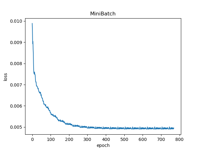
1 batch_size=5

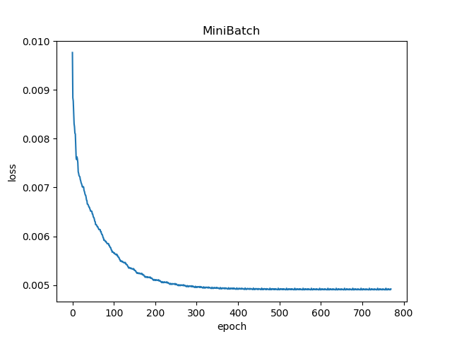
2 batch_size=10

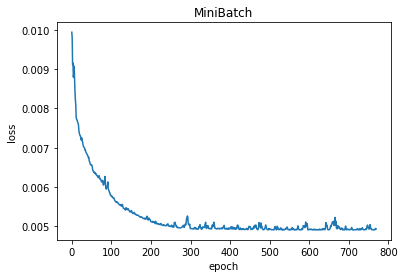
3 batch_size=15

Conclusion

当使用MiniBatch方法进行梯度下降时，可以发现batch_size对于interation次数有很大的影响（见下表），且该影响不是线性的，是跟数据的分布有关的。

batch_size	interation
5	21
10	5
15	8

改变MiniBatch选样本的策略，由顺序选取，改为随机选取

代码

def GetBatchSamples(X,Y,batch_size,iteration):
    num_feature = X.shape[0]
    bX = []
    i=0
    while i<batch_size:
        x = np.random.randint(0,X.shape[1])
        if x not in bX:
            bX.append(x)
            i+=1
    batch_x = X[0:num_feature,bX].reshape(num_feature,batch_size)
    batch_y = Y[0,bX].reshape(1,batch_size)
# #     start = np.random.randint(0,X.shape[1]-batch_size)
#     start = iteration * batch_size
#     end = start + batch_size
#     batch_x = X[0:num_feature,start:end].reshape(num_feature,batch_size)
#     batch_y = Y[0,start:end].reshape(1,batch_size)
    return batch_x, batch_y

Result

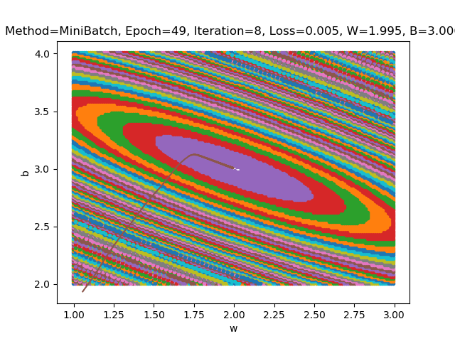
下图为 batch_size 为 10 时的 loss-epoch 图像和 loss-(w,b) 二维图像


下表显示 batch_size 为 10 时的 epoch 和 iteration 值（多次运行结果）

Number	Epoch	Iteration
0	37	14
1	26	1
2	34	0
3	43	8
4	39	3
5	40	15
6	32	5
7	48	5
8	47	8
9	36	8

可以发现随机选取batch样本时运行结果时好时坏差异非常大，但是总体来讲结果总是好于batch_size为5时的结果，说明小批量梯度下降表现比SDG更优秀。

关于损失函数的2D图像的问题：

1 为什么是椭圆而不是圆？

根据我们假设的函数\(y=w*x+b\)可以发现，此处的\(w\)和\(b\)二者的地位不对等，当在计算损失函数的时候，随着x的变化，\(w\)和\(b\)变化值不同，即\(dw\)和\(db\)不同。
\[db=\sum{\frac{z-y}{m}}\]\[dw=\frac{(z-y)*x^T}{m}\]

2 如何把这个图变成一个圆？

根据上一问的思路，我们可以发现只要让\(dw\)和\(db\)相同，就可以使图像变成一个圆。

根据这个思路，我们先假设函数为\(y=(x+w)+b\)，计算出来的损失函数图像变化相同了，但却不是一个圆，而是直线。

由此可见是构造函数的问题，我们应当使函数中w和b的地位对等但不相同（即否定了\(w+b\)或\(w*b\)这种形式）。

根据这一思路，我们可以构造出函数\(y=k+w*x_1+b*w_2\)，并且此处\(x_1\)和\(x_2\)的变化尺度应该相同（如范围都是\([0,10]\)）。这样既能保证\(w\)和\(b\)二者的地位对等，又能保证二者不相等，出来的图像就会是圆而不是椭圆。

3 为什么中心是个椭圆区域而不是一个点？

因为MiniBatch的梯度下降算法是求近似解的算法，而不是求其解析精确解的算法，这就意味着在函数的最底部\(w\)和\(b\)的取值会卡在一个小范围内反复跳跃，无法跳出这一个小范围，而这个小范围内的损失函数的结果也就会都相同。

【自问自答】4 如何缩小中心椭圆区域的范围？

第一种方法是缩小设置的误差值，如从10e-5变为10e-7，然而这种方法治标不治本。

第二种方法是调整\(\eta\)的值，使其能进入最后的小范围。